An Introduction to Geographic Information System
1 MODULE 1: Overview of the basic concept of Geographic Information System.
1.1 Objectives:
This module enables the students to:
Possess knowledge of the basic GIS concepts;
Gain knowledge about GIS data models and structures and;
Understand the Coordinate reference systems (CRS).
1.2 Outcomes:
After reading this module, students should be able to:
Define what is GIS;
Differentiate vector from raster;
Familiarized with the common Coordinate Reference Systems (CRS)
1.3 Definition of Terms
- Surveying
-
It is the art,science and technology of making all essential measurements to determine and establish the relative of points together with their physical and cultural details.
- Altitude
-
Used to describe the vertical and distance between an object and a reference points.
- Elevation
-
Used to describe the height of a place above sea level.
- Contour line
-
are imaginary line of a terrain that joins the points of equal elevation above sea given level,such as mean sea level or benchmark.
- Contour interval
-
The difference in values between contours.
NoteContour lines never cross each other and moving from one contour to another indicates change in elevation.
1.4 History of GIS
1.4.1 Early history of GIS (1960)
The field of geographic information systems (GIS) started in the 1960s as computers and early concepts of quantitative and computational geography emerged.
Early GIS work included important research by the academic community.
Later, the National Center for Geographic Information and Analysis, led by Michael Goodchild, formalized research on key geographic information science topics such as spatial analysis and visualization.
These efforts fueled a quantitative revolution in the world of geographic science and laid the groundwork for GIS.
1.4.2 The First GIS (1963)
Roger Tomlinson’s (the father of GIS) pioneering work to initiate, plan, and develop the Canada Geographic Information System resulted in the first computerized GIS in the world in 1963.
The Canadian government had commissioned Tomlinson to create a manageable inventory of its natural resources. He envisioned using computers to merge natural resource data from all provinces. Tomlinson created the design for automated computing to store and process large amounts of data, which enabled Canada to begin its national land-use management program.
He also gave GIS its name.
1.4.3 The Harvard Laboratory (1965)
While at Northwestern University in 1964, Howard Fisher created one of the first computer mapping software programs known as SYMAP. In 1965, he established the Harvard Laboratory for Computer Graphics.
While some of the first computer map-making software was created and refined at the Lab, it also became a research center for spatial analysis and visualization.
Many of the early concepts for GIS and its applications were conceived at the Lab by a talented collection of geographers, planners, computer scientists, and others from many fields.
1.4.4 ESRI is Founded (1969)
In 1969, Jack Dangermond—a member of the Harvard Lab—and his wife Laura founded Environmental Systems Research Institute, Inc. (Esri).
The consulting firm applied computer mapping and spatial analysis to help land use planners and land resource managers make informed decisions.
The company’s early work demonstrated the value of GIS for problem solving. Esri went on to develop many of the GIS mapping and spatial analysis methods now in use. These results generated a wider interest in the company’s software tools and work-flows that are now standard to GIS.
1.4.5 GIS Goes Commercial (1981)
As computing became more powerful, Esri improved its software tools.
Working on projects that solved real-world problems led the company to innovate and develop robust GIS tools and approaches that could be broadly used.
Esri’s work gained recognition from the academic community as a new way of doing spatial analysis and planning.
In need of analyzing an increasing number of projects more effectively, Esri developed ARC/INFO—the first commercial GIS product. The technology was released in 1981 and began the evolution of Esri into a software company.
1.5 Basic GIS Concept
This module aims to provide a discussion about basic Geographic Information System (GIS). The discussions about GIS in this module are not comprehensive and are intended for beginner students. Further readings and resources are provided at the end of this module for students who wish to learn more about the science and art of GIS.
Through the years, the improvement and development of computers has revolutionized map making. This revolution helped cartographers to shift from tedious hand-drawn maps to digital maps. GIS allows anyone to visualize spatial data in space and in an interactive manner.
Geography is a core and essential element at the heart of GIS. By definition, it means the study of locational and spatial variation in both physical and human phenomena on earth(Balasubramanian 2014). In other words, one cannot fully grasp or implement GIS without considering the principles and concepts of geography.
In the context of GIS, geography refers to the spatial relationships and characteristics of features on the Earth’s surface.
By utilizing GIS, it is possible to incorporate a geographical aspect to any data by linking it to specific locations. This is accomplished through techniques such as Geo-tagging and Geo-referencing. Data or information that is tied to a specific location is referred to as geospatial.
1.5.1 What is Geographic Information System (GIS)
GIS is a computer-based system that is designed to capture, manipulate, analyze, manage, retrieve, and display all types of geographically reference data.
The keywords are: Computer-based, System, and geographically-referenced.
The primary function of GIS is not just to create maps but also to display data in a spatially explicit manner. This enables users to identify emerging patterns and gain a better understanding of phenomena.
1.5.2 Comparison between GIS and Mapping
GIS is often associated with maps, but it is important to understand that it encompasses much more than just mapping. While maps are a way to display data in a spatially explicit manner, GIS is a broader concept that includes many different applications. In fact, GIS is an umbrella term that refers to a variety of tools and techniques used to analyze, manage, and visualize geospatial data.
GIS is ” Mapping plus more”
1.5.3 GIS as a System
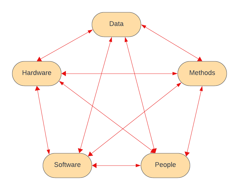
GIS may appear as a single entity, but it is actually a system consisting of a collection of components working together to perform a particular function. As a system, GIS comprises various elements connected and integrated in a cohesive manner. Like any other system, GIS is composed of numerous components, including but not restricted to:
|
|
|
|
|
|
GIS as a system is a complex network of organized and interconnected elements which includes the following: a.) Physical (hardware, people, print maps) b.) Intangible (methods, procedures, digital data).
1.5.4 The Concept of Geospatial Data
Geospatial data refers to any data that has a location component and can be displayed digitally.
The prefix “Geo” suggests “Earth” while “Spatial” comes from the root word “Space”. The term “Features” is also sometimes used to refer to the vector type of GIS.
In geospatial data, anything occurring on, above, or below the Earth’s surface is included. The term is often used interchangeably with spatial data or GIS data.
|
|
|---|---|
|
|
|
|
1.5.5 GIS Data Models
There are two general types of data in GIS these are “Vector” and “Raster”.
1.5.5.1 Raster
The raster data model, along with the vector data model, is one of the earliest and most widely used data models within geographic information systems (Tomlin 1990). It is typically used to record, analyze, and visualize data with a continuous nature such as elevation, temperature, or reflected or emitted electromagnetic radiation. The term raster originated from the German word for screen, implying a series of orthogonally oriented parallel lines.
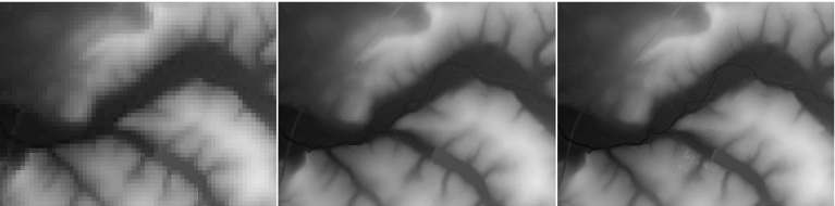
1.5.5.2 Pixels and Resolution
Each tiny square of information in a digital image is called a Pixel. These Pixels, or “cells,” are responsible for representing features on, above, or below the earth’s surface. Unlike vectors, rasters are resolution-dependent. This means that the quality of the data is influenced by the size and number of Pixels used to cover a fixed unit area.
When you zoom-in very closely on a digital image, the amount of detail you see is determined by the size of the Pixels. The resolution is dictated by the pixel size expressed in ground units, as determined by the Coordinate Reference System (CRS).
“Picture Element” or “Pixel” is the smallest unit of information in a raster.
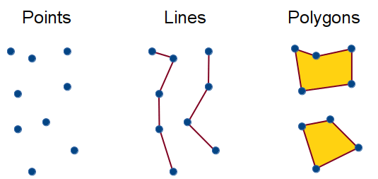
1.5.5.3 Vector
Vector data models represent spatial features using points and their associated X, Y coordinate pairs, similar to a hand-drawn map. There are three types of vector data these are Points, Lines, and Polygons.
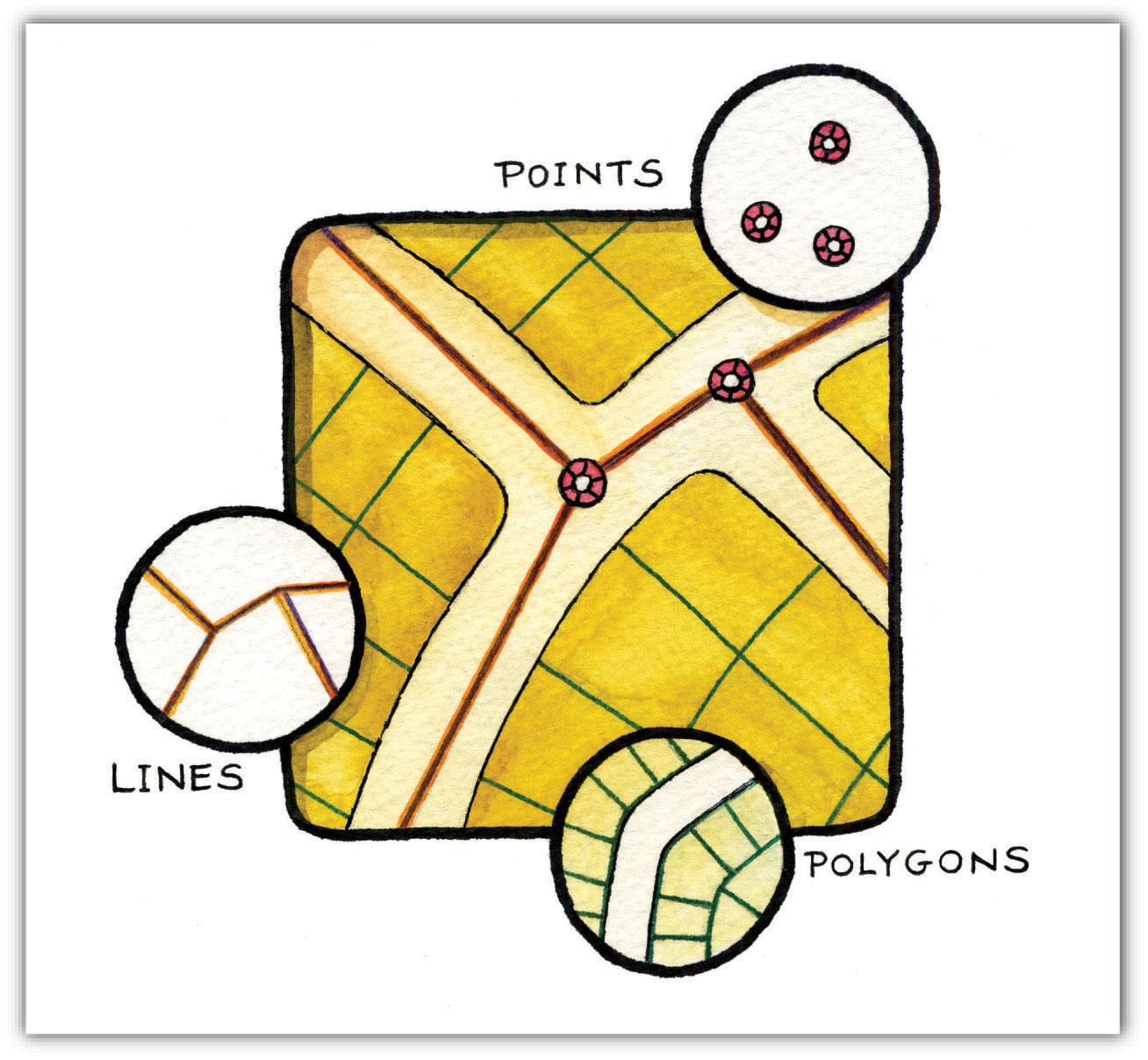
- Points
-
A zero-dimensional object containing a single coordinate pair. In a GIS, points have only the property of location.
- Lines
-
are one-dimensional features composed of multiple, explicitly connected points. Lines are used to represent linear features such as roads, streams, faults, boundaries, and so forth.
- Polygon
-
are two-dimensional features created by multiple lines that loop back to create a “closed” feature. In the case of polygons, the first coordinate pair (point) on the first line segment is the same as the last coordinate pair on the last line segment.
The appropriate type of vector to use depends on the objector entity of interest.
1.5.6 The Shapefile
It is the most common supported vector file format. Despite the name, this is not a single file but a group of files sharing the same name but with different file extensions.
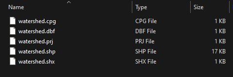
| File format | Description |
|---|---|
| .shp |
|
| .prj |
|
| .dbf |
|
| .shx |
|
| .qml |
|
1.5.7 File formats for Vector and Raster
Digital files come in various file formats, which can be identified by the suffixes following the “dot” (e.g. *.tiff). In the field of Geographic Information Systems (GIS), the following file types are the most common and widely accepted. The formats written in bold letters are the most popular file types used in GIS.
| GIS Data Model | Common file format |
|---|---|
| Raster |
|
| Vector |
|
KML is a file that can be created, visualized, and edited using Google Earth application. SHP is the standard format for vector files and can be opened and read by almost any GIS software.
1.5.8 Examples of Vector and Raster
Below are some of the examples of vector and raster data. Note that this is not a comprehensive list.
| Data Model | Examples | Sample Products |
|---|---|---|
| Raster |
|
|
| Vector |
|
|
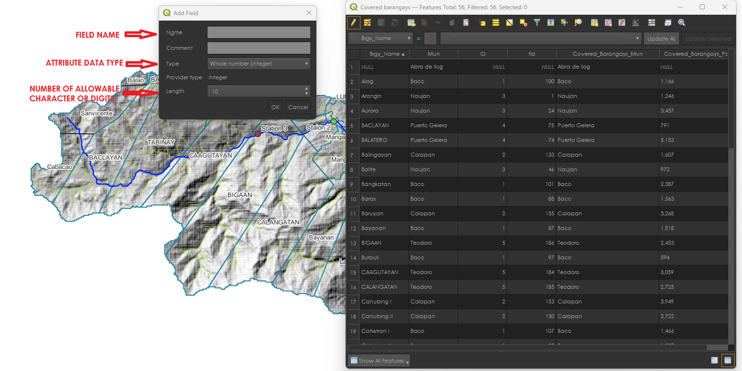
1.5.9 Attributes
Every data, especially vector data, has an associated attribute table that holds information about that data. These could most easily be understood if the data is considered as a spreadsheet with one row per feature and one column.
Columns are also called Fields
Rows are also called Data/Records
Vector data is usually linked with attributes, which can be modified by adding or removing fields, requiring the definition of their data type. The attribute’s type will vary depending on the values expected to be stored in the cells of that field.
Rows are added when a feature or polygon is drawn from the QGIS map area.
1.5.10 Coordinate Reference System (CRS)
Do you still remember the Cartesian Coordinate System? This system allows us to locate the position of any point in space relative to an origin, which is the intersection of two perpendicular lines.
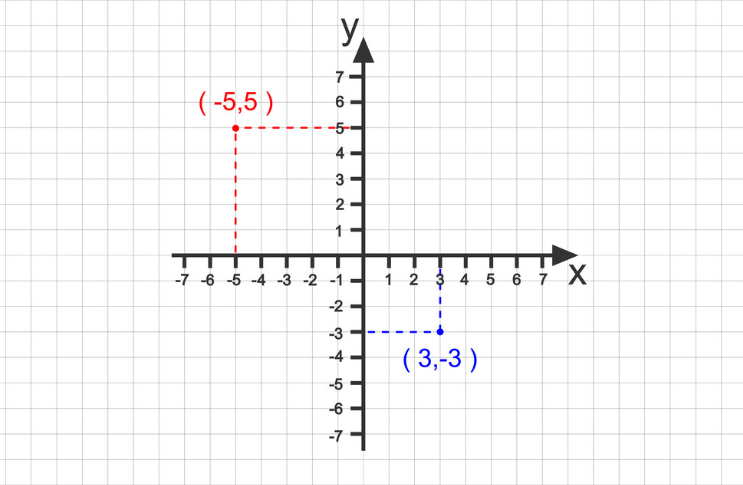
The principles of the Cartesian Coordinate System is the same principle used in locating places on earth.
Any point on earth’s surface can be represented by longitude and latitude instead of X and Y axes. The longtitude and latitude divided the earth vertically and horizontally in such a way that any given point could be NorthSouth or WestEast. Any point is relative to the Longtitude-Latitude intersection, which is the zero-degree Longtitude (Prime Meridian) and zero-degree Latitude (Equator).
1.5.11 Types of Coordinate Reference Systems (CRS)
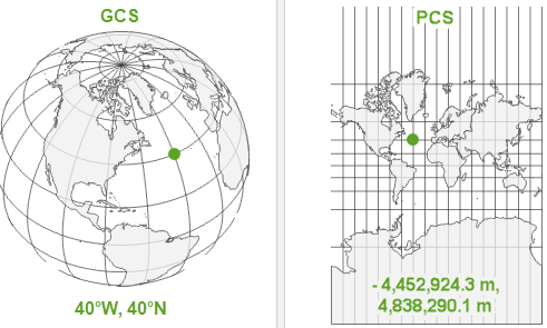
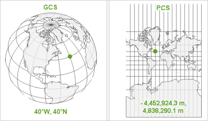
There are two most commonly used coordinated reference systems in GIS. The Geographic Coordinate Systems (GCS) and the Projected coordinate systems (PCS). These two CRS display GIS data differently on a computer.
The CRS, or Coordinate Reference System, is responsible for determining the units of measurement in a map, whether it’s angular or linear. It also impacts the ability of map layers to overlay with one another. As a general rule, all data sets should have the same CRS to ensure proper alignment of the layers.
1.5.12 The Geographic Coordinate Systems (GCS)
The GCS uses the longitude latitude system and uses three-dimensional spherical surface to find locations and points since positions are based on angular distances everything is measured in degree units.
A location on Earth is defined by its coordinates, known as longitude and latitude. These coordinates are angles that originate from the Earth’s center and extend to a specific point on the planet’s surface. Typically, these angles are quantified in degrees or grads.
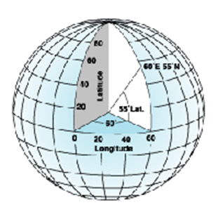
Within the spherical coordinate system, the horizontal or east-west running lines represent parallels, which are lines of constant latitude. Conversely, the vertical or north-south running lines signify meridians, which are lines of constant longitude. Together, these lines wrap around the Earth, creating a grid-like pattern known as a graticule.
The equator is the central line of latitude, equidistant from both poles, and is designated as the zero latitude line. The prime meridian, which is the zero longitude line, typically runs through Greenwich, England in most Geographic Coordinate Systems (GCSs). The point where the equator and the prime meridian intersect is known as the graticule’s origin, with coordinates (0,0).
Latitude and longitude coordinates are conventionally expressed in decimal degrees or as degrees, minutes, and seconds (DMS). Latitudes are gauged from the equator, extending from -90° at the South Pole to +90° at the North Pole. Longitudes, on the other hand, are gauged from the prime meridian, spanning from -180° westward to 180° eastward. For instance, given that the prime meridian crosses Greenwich, England, Australia’s position—south of the equator and east of Greenwich—results in positive longitude and negative latitude values.
Thinking of longitude as the ‘x’ value and latitude as the ‘y’ can be useful. When data is plotted on a geographic coordinate system, it’s treated as though each degree is a fixed unit of measurement, akin to the Plate Carrée projection. It’s important to note that a single physical location may be represented by different coordinate values across various geographic coordinate systems.
There are at least three ways to express GCS:
Degrees-Minutes-Seconds
Decimal minutes
Decimal degrees
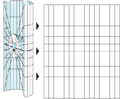
1.5.13 Projected Coordinate Systems
A Projected Coordinate System (PCS) is established on a plane, which is a flat, two-dimensional surface. In contrast to a Geographic Coordinate System (GCS), a PCS maintains consistent lengths, angles, and areas throughout its two dimensions. A PCS invariably relies on an underlying GCS, which itself is derived from a spherical or spheroidal shape. Beyond the GCS, a PCS encompasses a map projection, which is further tailored for specific locations through a collection of projection parameters, and it also specifies a linear unit for measurement.
1.5.14 Geographic (datum) transformations
When dealing with two datasets that are aligned to different geographic coordinate systems, a geographic (datum) transformation may be necessary. This transformation is a precise mathematical process used to translate coordinates from one geographic coordinate system to another. Much like the coordinate systems themselves, there is an extensive array of predefined geographic transformations available for use. It’s crucial to apply the correct geographic transformation when required, as failure to do so can result in coordinates being misplaced by as much as several hundred meters. In cases where a direct transformation is not available, it may be necessary to employ an intermediary GCS, such as the World Geodetic System 1984 (WGS84), and perform a combination of two transformations.
“Easting” refers to the measure of how far east a point is from the origin within a coordinate system, quantified in the units of that system. It corresponds to the x-value in a rectangular coordinate system. “Northing,” on the other hand, denotes the measure of how far north a point is from the origin, also measured in the system’s units, aligning with the y-value in a rectangular coordinate system.
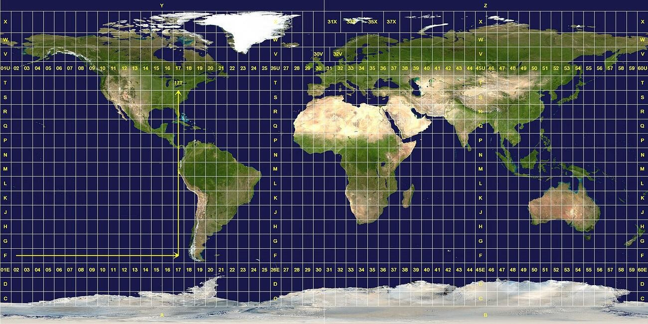
The world is divided into 60 longitudinal projection zones, which are sequentially numbered from 1 to 60, beginning at 180°W. Each zone spans 6 degrees in width, with certain exceptions in regions like Norway and Svalbard where the zones differ in width.
Comparison between PCS and GCS
A GCS is round, and so records locations in angular units (usually degrees). A PCS is flat, so it records locations in linear units (usually meters).
Once your dataset is prepared to be depicted, it must determine the method of portrayal. The dilemma arises from the discrepancy between the spherical nature of the Earth’s surface—and consequently, your Geographic Coordinate System (GCS)—and the planar characteristics of your map and computer display. Transferring the Earth’s curvature onto a flat medium inevitably leads to distortion. It’s akin to attempting to flatten an orange peel on a table; it nearly works, but not without some tearing. This is where the utility of map projections is evident. They provide instructions on how to manipulate the Earth’s representation—how to strategically tear and stretch that orange peel—so that the most crucial aspects of your map suffer minimal distortion and are optimally represented on the map’s flat plane.
2 MODULE 2: INTRODUCTION TO QGIS (Installation, User-Interface, and Plugins)
2.0.1 Objectives:
This module enables the students to :
Have an overview on what is QGIS and ,
Familiarize its user interface.
2.0.2 Outcomes:
After reading and following the steps and procedure in this module, the students should be able to:
Install QGIS in their computer successfully,
Familiarized its user interface, able to identify useful geoprocessing icons and,
Install plug-ins.
2.1 Overview of the QGIS Software
2.1.1 What is QGIS?
QGIS is a sophisticated GIS application that not only stands on the shoulders of Free and Open Source Software (FOSS) but also takes pride in being part of the FOSS community.
QGIS is an accessible and open-source Geographic Information System (GIS), licensed under the GNU General Public License. As an esteemed project of the Open Source Geo-spatial Foundation (OSGeo), it operates across various platforms including Linux, Unix, Mac OSX, Windows, and Android, and accommodates a wide array of vector, raster, and database formats and capabilities.
2.1.2 QGIS Applications
QGIS is not only a desktop GIS. It can also be used for spatial file browser, a server application, and web applications. Below are some of the applications of QGIS.
| Application | Description |
|---|---|
| QGIS Desktop | Create, edit, visualise, analyse and publish geospatial information. For Windows, Mac, Linux, BSD and Android. |
| QGIS Server | Publish QGIS projects and layers as OGC compatible WMS, WMTS, WFS and WCS services. Control which layers, attributes, layouts and coordinate systems are exported. QGIS server is considered as a reference implementation for WMS 1.3. |
| QGIS Web Client | Publish QGIS projects on the web with ease. Benefit from the powerful symbology, labeling and blending features to impress with your maps. |
| QGIS on mobiles and tablets | The QGIS experience does not stop on the desktop. Various third-party touch optimized apps allow you to take QGIS into the field |
2.1.3 Software Installation
The following steps shows you how to install QGIS into your computer. In order to install the QGIS software you need to download the software first.
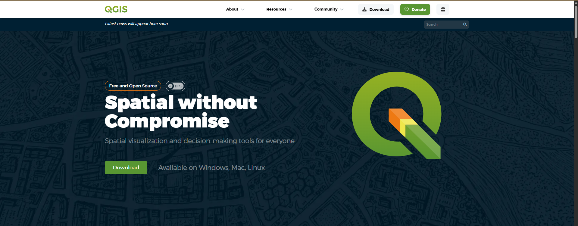
Step 1. In your internet browser type https://qgis.org/en/site/index.html in the search bar. The official website of QGIS will appear.
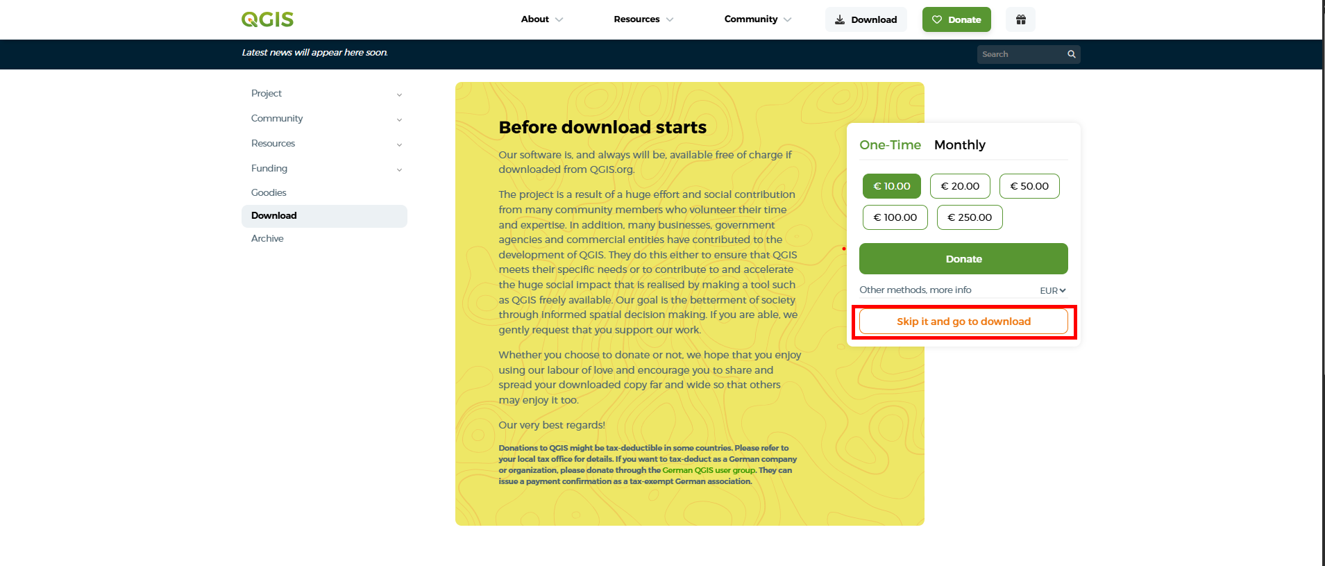
Step 2. After clicking the Download button, it will re direct you to the download page. Click Skip it and go to download button.
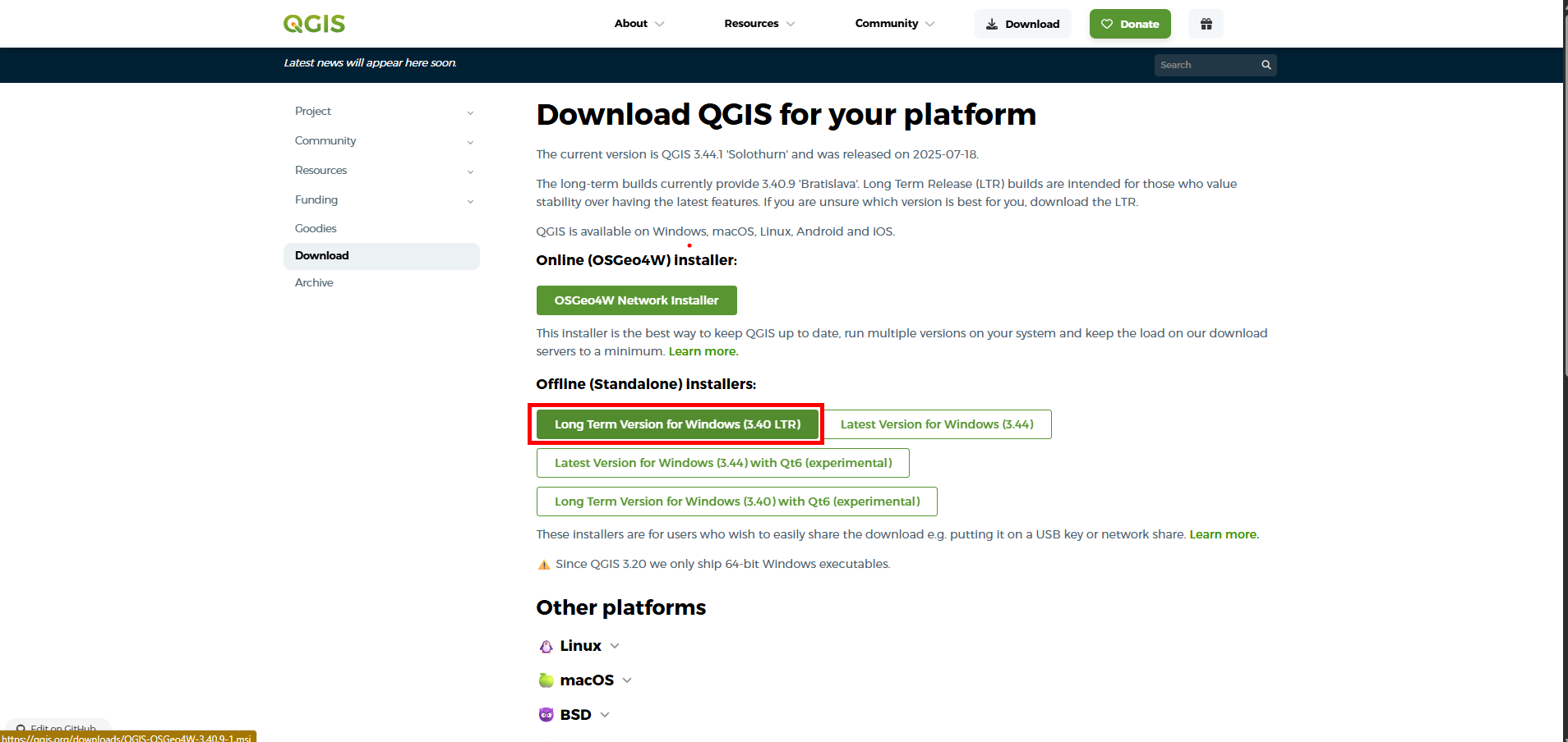
Release Candidate (RC) is the latest version of QGIS that is being tested and can be used. The only disadvantage of this version is that it is prone to Bugs and frequent Crash. While Long Term Release (LTR) is usually older version of the software that is more stable that the release candidate.
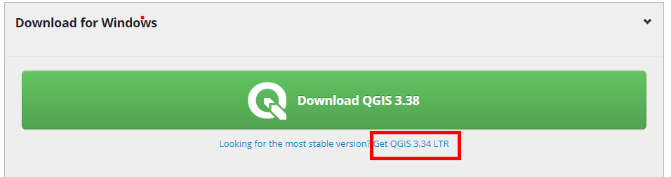
Step 3. The download page will appear showing a large download button. Click the ![]() link below the button since it is better to download the long term release version of the software.
link below the button since it is better to download the long term release version of the software.
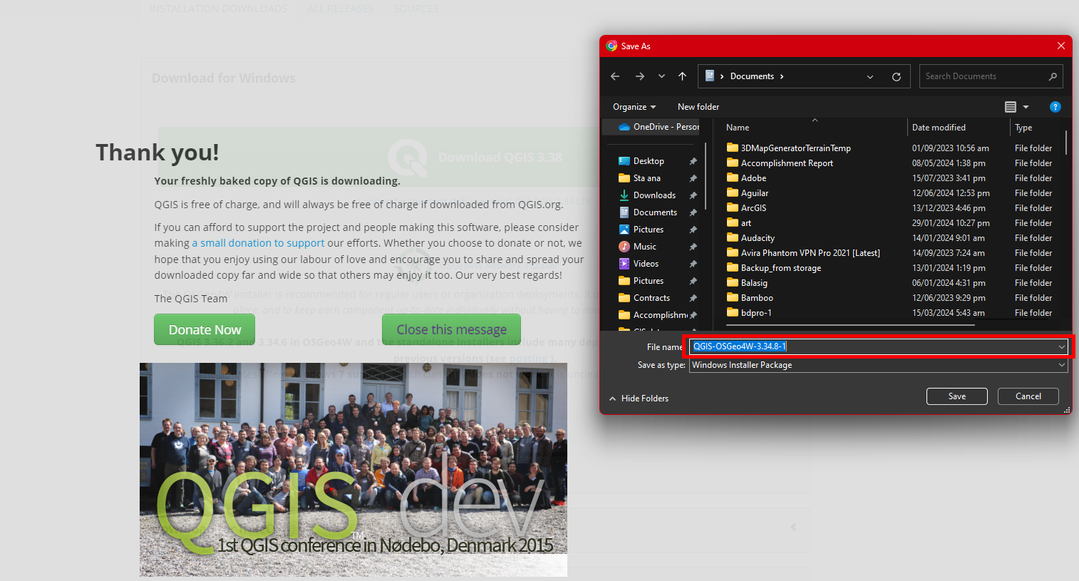
Step 4. A dialog box will appear asking you where to put the downloaded file. Choose a folder then click ![]() button to download the software. Wait until the software is downloaded. This may take some time depending on the size of the file being downloaded and how fast your internet connectivity.
button to download the software. Wait until the software is downloaded. This may take some time depending on the size of the file being downloaded and how fast your internet connectivity.
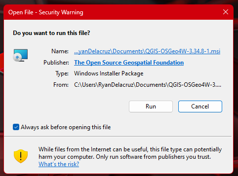
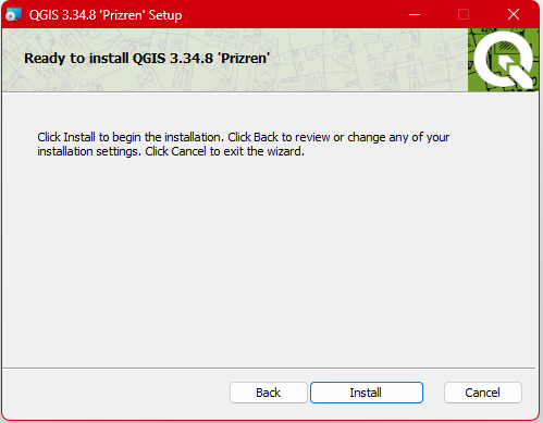
Step 5. Double click the file that you have downloaded and a dialog box will appear. Click ![]() and another dialog box will appear. Just click
and another dialog box will appear. Just click ![]() and tick the
and tick the  lastly , hit
  . Wait Until the software is successfully installed.
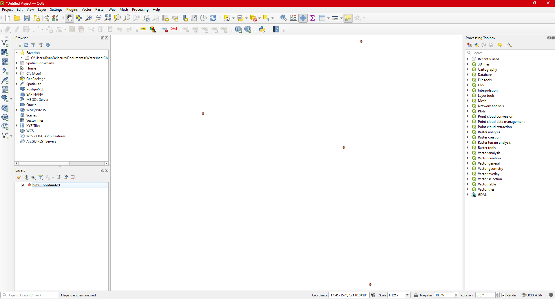
2.1.4 QGIS Graphical User Interface (GUI)
After installing the software, click the windows icon ( ![]() windows icon) and look for the recently installed application or type QGIS Desktop 3.34.8 on search bar (
windows icon) and look for the recently installed application or type QGIS Desktop 3.34.8 on search bar (![]() search bar ).
search bar ).
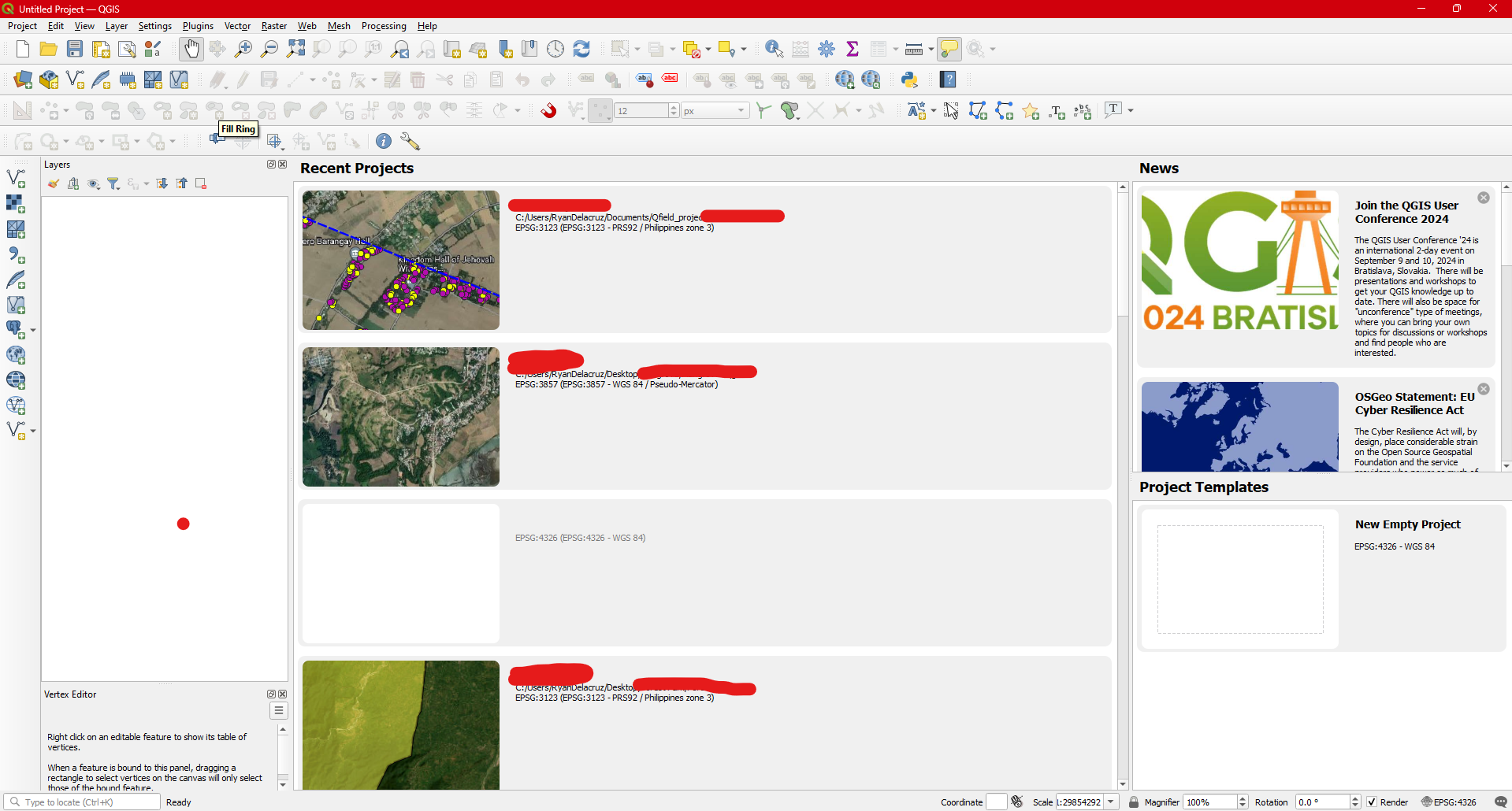
Step 1. Click  to open the software. The QGIS interface will show up showing your recent project if you have already used it but usually this will be blank if you are using it for the first time.
Step 2. Press Ctrl + N to start a new project or Click the 
 icon. A new untitled project was just created.
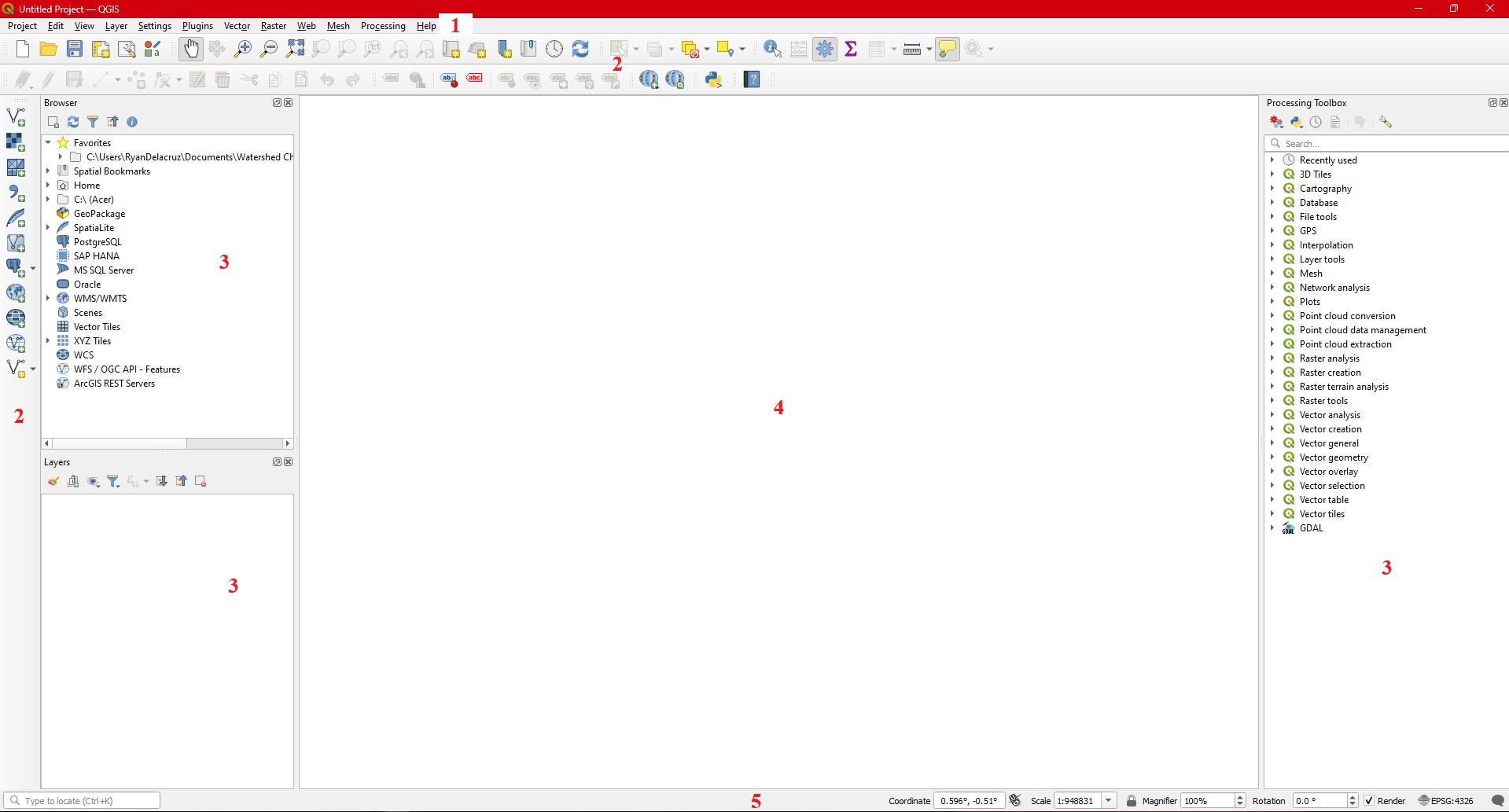
| Component | Description |
|---|---|
|
The Menu bar provides access to QGIS functions using standard hierarchical menus. |
|
The toolbars provide access to most of the functions in the menus, plus additional tools for interacting with the map. |
|
QGIS provides many panels. Panels are special widgets that you can interact with (selecting options, checking boxes, filling values…) to perform more complex tasks. |
|
The map view provide visualization of the layers being loaded into the QGIS. |
|
The status bar provides you with general information about the map view and processed or available actions, and offers you tools to manage the map view. |
A more detailed information on each of the component can be access from the official website of QGIS.
3 MODULE 3: LOADING DIFFERENT DATA MODELS INTO QGIS
3.0.1 Objectives:
This Module enables the students to:
Differentiate different data models,
Load different data into QGIS.
3.0.2 Outcomes:
After reading and following the steps and procedure in this module, the students should be able to:
Gain knowledge about the different data models,
Confidently load different data models into QGIS.
3.1 Loading Vector Layers
The data to be use for this exercise can be downloaded here.
3.1.1 Loading a . csv file
A .csv file stands for comma-separated values file. It’s a simple and widely used format for storing tabular data in plain text. Each piece of data in the file is separated by a comma (,). This makes it easy for computer programs to read and understand the data.
The following steps will guide you on how to load .csv files into QGIS.
Step 1. Open you QGIS software and on the Manage layers Toolbars Click  Add delimited text icon or Press
 CTRL + SHIFT + T.
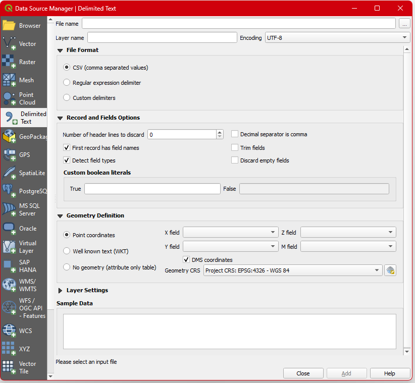
Step 2. On the right of the File name textbox there is a button with three dots, Click  to browse for the location of your .csv file.

Step 3. In your Mapping data set folder, Left Click on Site Coodrinate1 and click Open. Your .csv file data will be loaded.
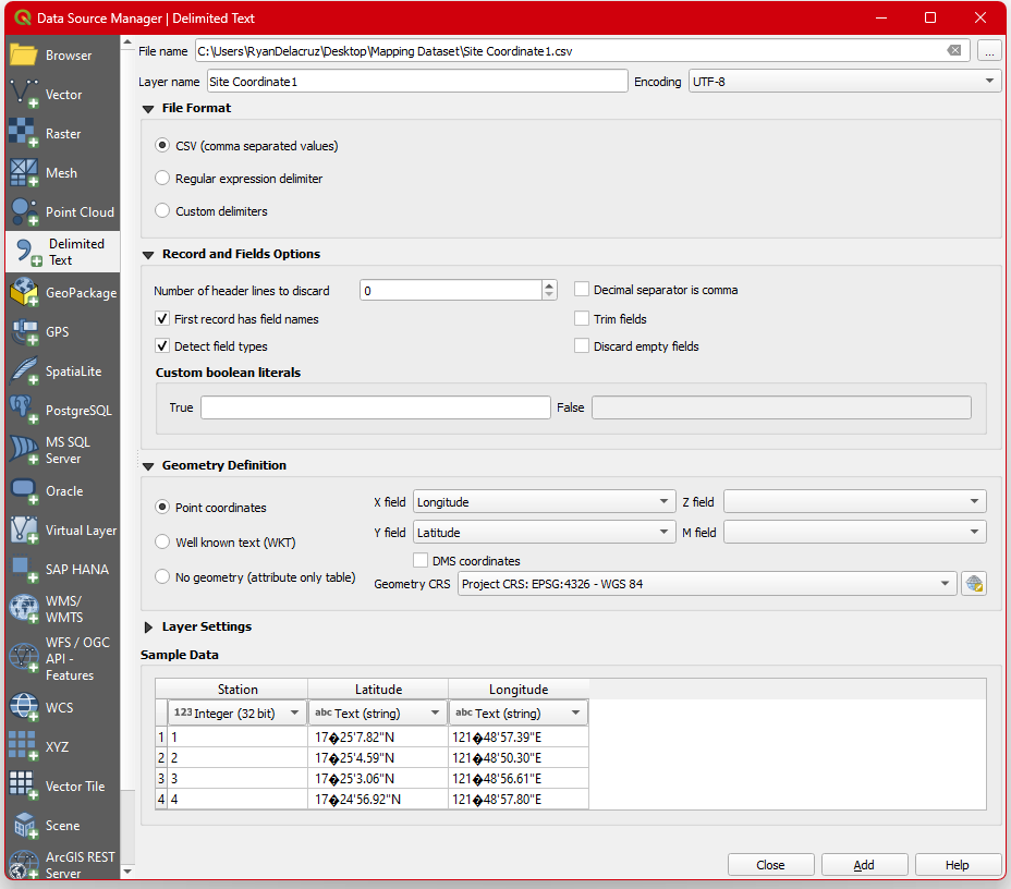
Your X and Y fields will automatically load the longitude and latitude data from your csv file. But there are instances that it does not load properly. You need to set it manually.
Step 4. Since your data is in Degrees Minutes Seconds, this will give you a hint that your csv file CRS is Geographic Coordinate format. Under the X and Y field check the  and Set the
 Geometry CRS to EPSG: 4326-WGS 84 .

Your Geometry CRS should be the same as your Project CRS to display the data properly.

Step 5. Click  button and hit
  . Your csv data should be loaded as points in the Map frame and will appear on the Layers Panel.
To Familiarized yourself about the process above, your next task is to load the Site Coordinate2.csv into your map window using the same steps. Take note of the CRS of the file and make sure your project CRS is the same as your layer CRS. Explore other ways to load csv files into QGIS.
3.1.2 Loading a shapefile
We have discussed in the previous module, that shapefile is not a single file but rather composed of a group of files sharing the same name but with different file extensions.
The following steps will show you how to load shapefiles into QGIS.
Step 1. In the Manage layer toolbar, Click  add vector layer icon or press
 CTRL + SHIFT + V and
a dialog box will appear.
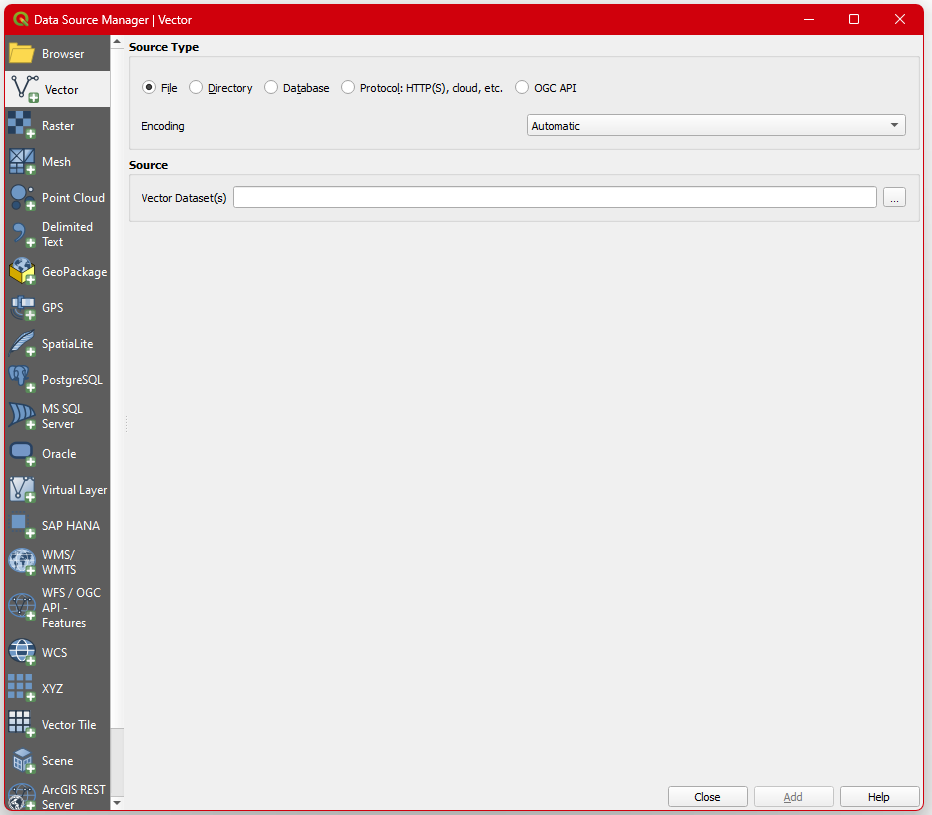
Step 2. Click the  browse button to look for your mapping data set folder.
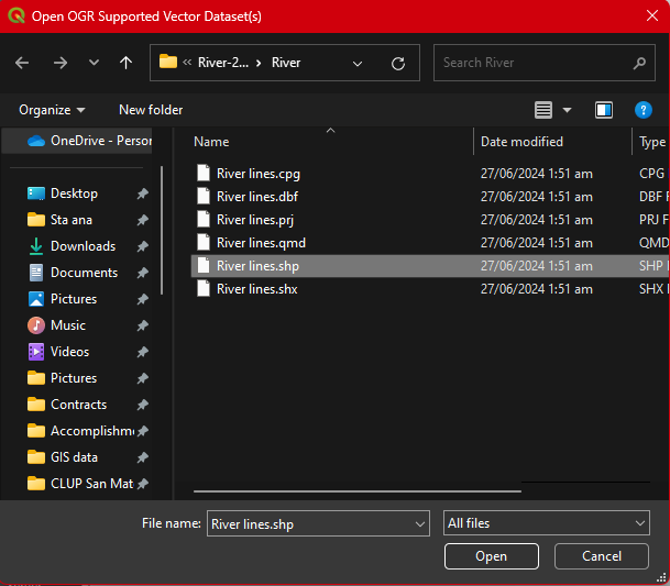
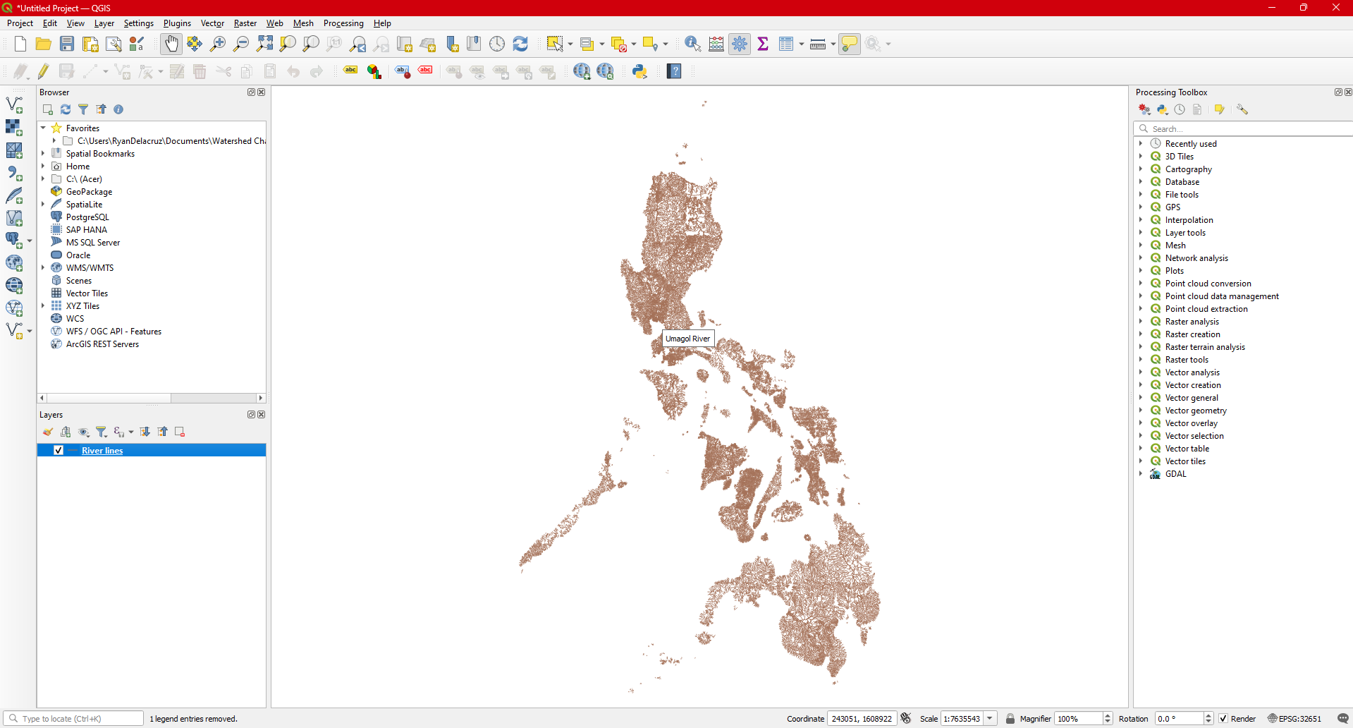
Step 3. In your data set, Click River lines.shp only and hit Open.
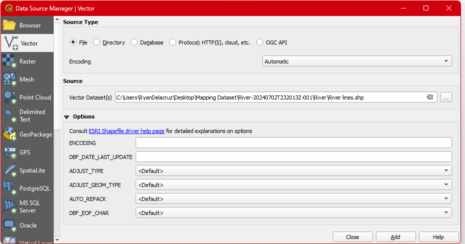
Step 4. After loading your shapefile hit  then
then  the dialog box. Your
 River lines Will now be added to the Layers Pannel.
3.2 Loading Raster Data
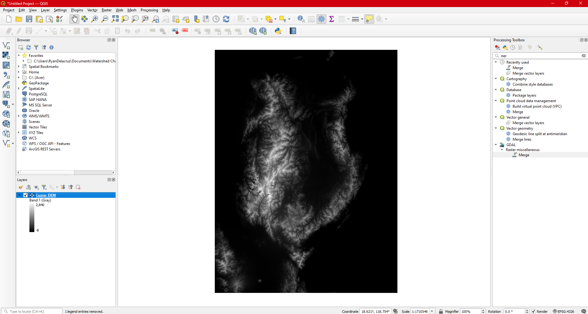
3.2.1 Loading Digital Elevation Model (DEM)
One of the most common raster data being use for geospatial analysis is the Digital Elevation Model (DEM). A digital elevation model (DEM) is essentially a 3D computer representation of Earth’s (or any celestial body’s) surface, focusing on elevation.
The following steps will guide you on how to load raster specifically DEM to QGIS.
Step 1. In the Manage Layers Toolbar Click the  add raster icon or press
 CTRL + SHIFT + R.
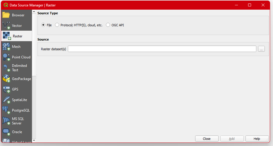
Step 2. Click the  browse button, and select and open the
 Luzon_DEM.tif file.
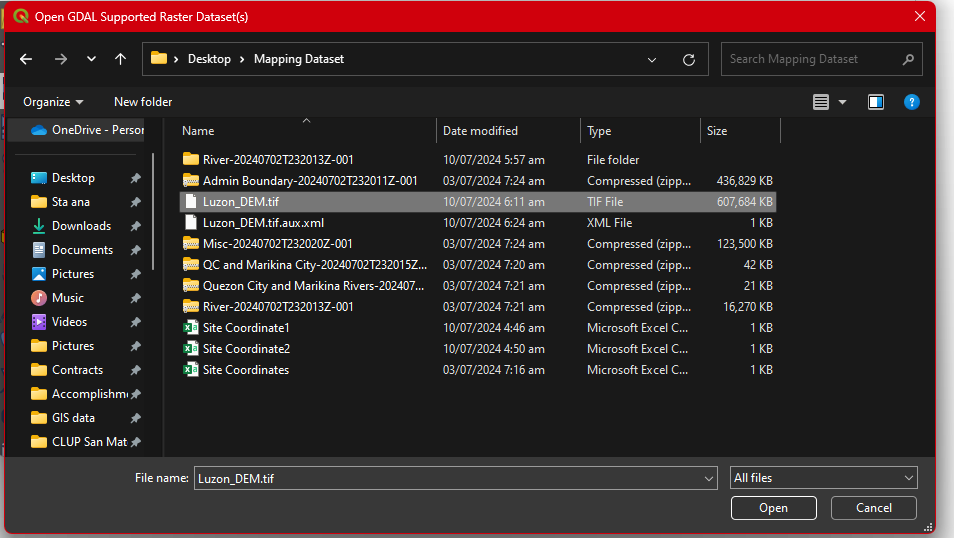
Step 3. Hit  then
then  the dialog box. Your DEM data is now loaded in the layers panel and in the map frame.
3.2.2 Loading Geotagged Photos from GeoCam App
GeoCam is a free mobile app that allows users to measure geographical data, like compass orientation, inclination, elevation, and overlay that information onto photos and videos of the surrounding area. A very helpful video tutorial on how to setup the application and on how to use the application can be access here.
For this module, we will assume that you have already gathered geotag photos from field works. A sample geotag photos data can be access here.
To load a geotaggedphoto follow these steps:
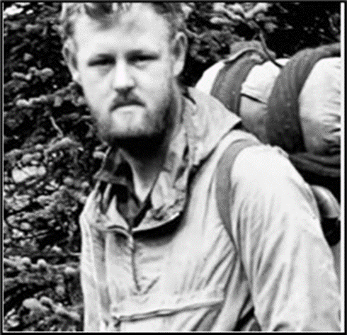
Step 1. Before loading the geotagged photo, it is very important to check what type of CRS the geotagged photo has. This is so, to ensure that your project CRS and your layer CRS are the same and to avoid errors when displaying the location of your geotagged photos.
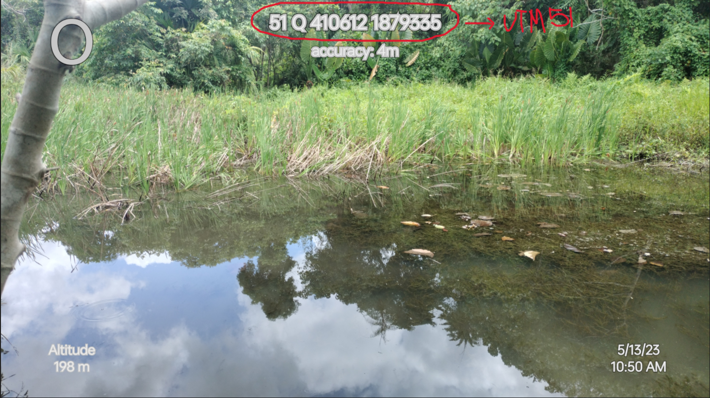
As you can see on the above sample geotagged photo, it’s CRS is UTM 51 as indicated on the first two digit number on the left of the coordinate. 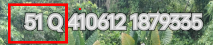
Step 2. After opening your QGIS Software, and after checking the geotaggedphoto’s CRS set your Project CRS to EPSG: 32651 - UTM zone 51N.
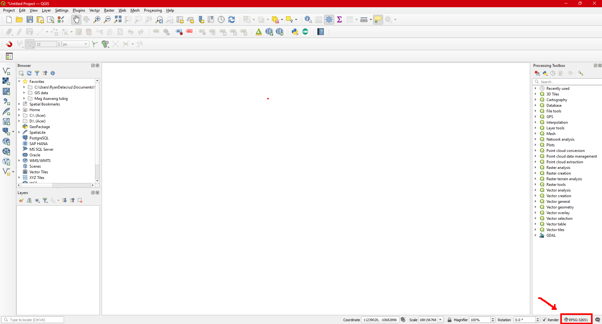
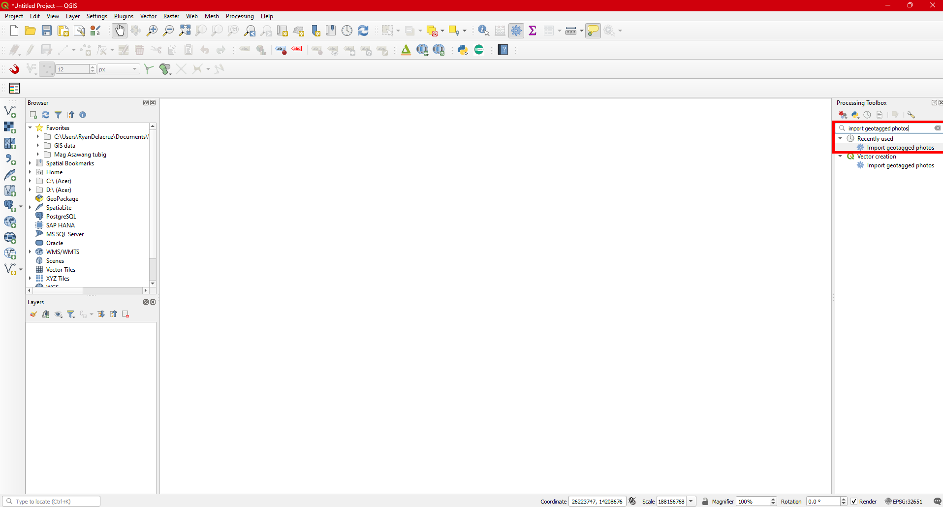
Step 3. To load the geotaggedphotos, under Processing Toolbox, type in Import Geotagphoto in the Searchbox. Select it and Double click on it to open the tool.
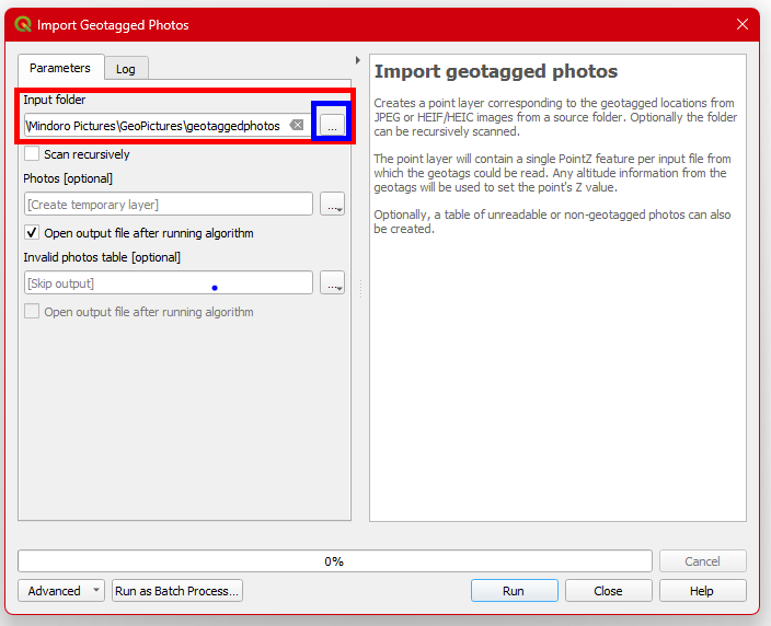
Step 4. In the Input folder, click  the
the browse button to look for the folder where you put all the geotaggedphotos you’re going to import. After finding the folder, click Run.
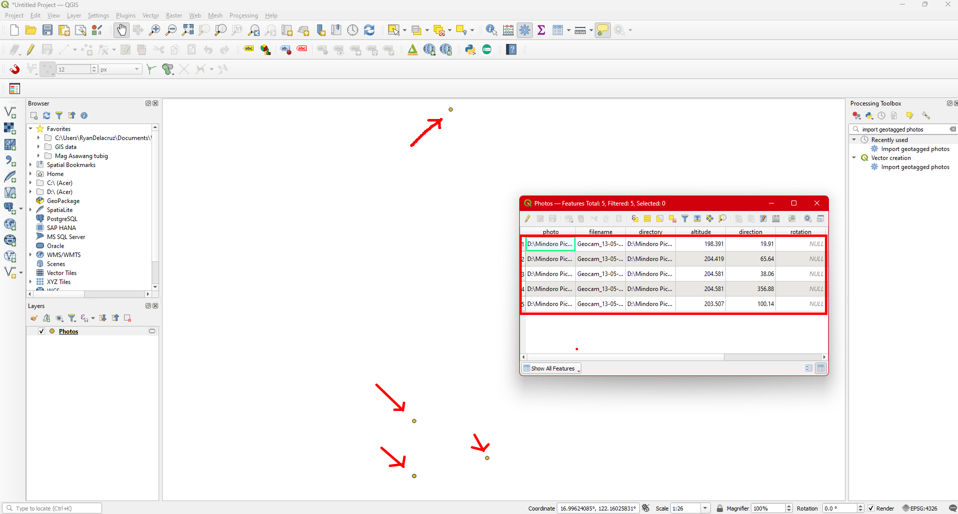
Step 5. After Clicking Run you can now see that the x and y coordinate of each photo is now converted in to points and a new layer name Photo is now visible on the Layers Panenl .
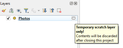
Remember to save the output since it is only temporary. Once you quit QGIS the layer will be remove and you need to load it again and follow the same process. To make it permanent , follow the same principles used in Step 4. in the Vector Analysis under the Clip exercise.
4 MOULE 4. MAP LAYOUT
4.0.1 Objectives
This module enables the students to:
Familiarize the QGIS Map composer.
Understand the different map elements.
4.0.2 Outcomes
After following the steps in this module, the students will be able to:
Composed and design their own Map.
Export their own Map into image.
4.1 Essential Map Elements
Maps are typically designed for audiences who aren’t GIS experts, such as politicians, citizens, or students. To effectively convey spatial information to these viewers, maps should include key elements like a title, map body, legend, north arrow, scale bar, acknowledgments, and a border.
Additional elements like a graticule or map projection can enhance map clarity. These elements, along with the title, legend, and other components, assist the viewer in understanding the map’s information. While the map body is central, these supporting elements aid in orientation and interpretation. For instance, the title identifies the subject, and the legend connects symbols to the data.
| Element | Description |
|---|---|
| Title | The map title is very important because it is usually the first thing a reader will look at on a map. |
| Map Border | The map border is a line that defines exactly the edges of the area shown on the map. |
| Map legend | A map is a simplified representation of the real world and map symbols are used to represent real objects. |
| North arrow | A north arrow (sometimes also called a compass rose) is a figure displaying the main directions, North, South, East and West. On a map it is used to indicate the direction of North. |
| Scale | The scale of a map, is the value of a single unit of distance on the map, representing distance in the real world. The values are shown in map units (meters, feet or degrees). The scale can be expressed in several ways, for example, in words, as a ratio or as a graphical scale bar. |
| Acknowledgement | In the acknowledgment area of a map it is possible to add text with important information. |
| Graticule | A graticule is a network of lines overlain on a map to make spatial orientation easier for the reader. |
| Name of Map Projection | A map projection tries to represent the 3-dimensional Earth with all its features like houses, roads or lakes on a flat sheet of paper. |
.jpg)
4.2 Using the Print Layout
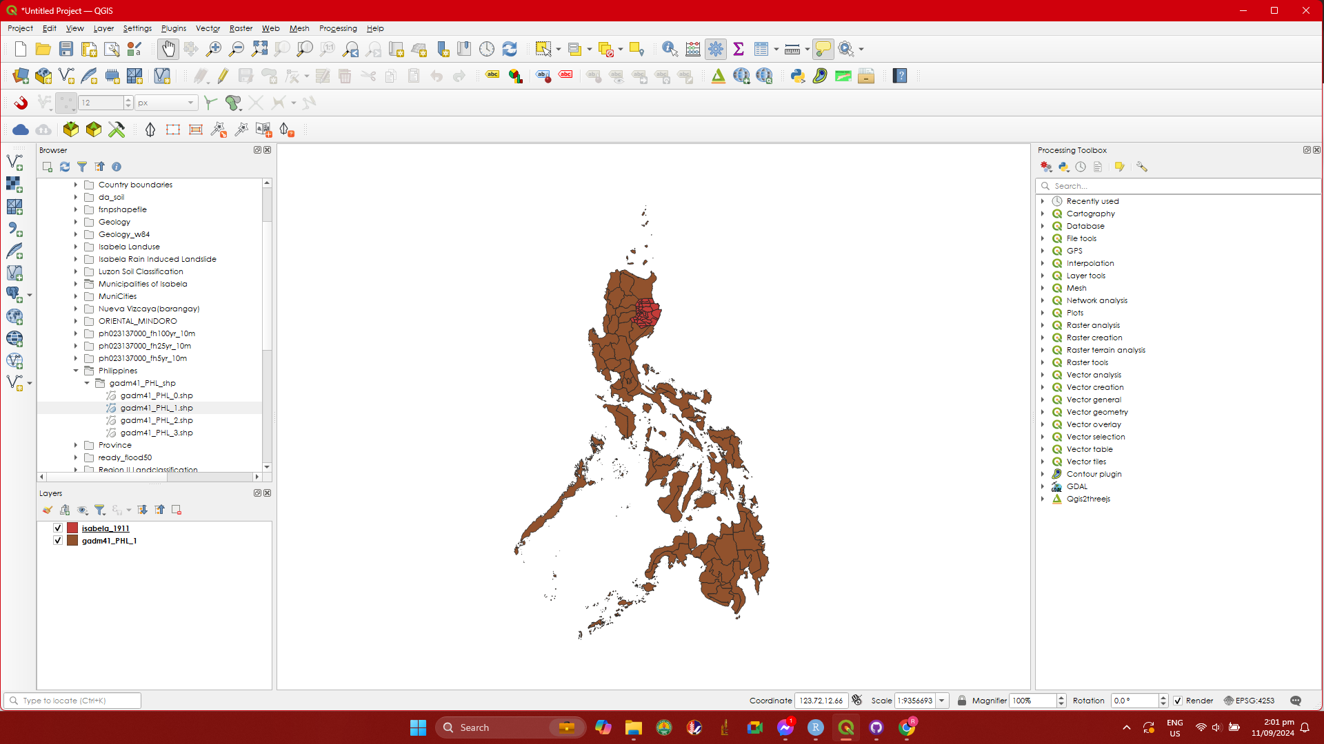
This steps will guide you oh how to produce your maps using the print layout. In order to use the layout, you must first load data into QGIS. Follow the steps above to load any recognized data model in QGIS. For this module we will create a map of the different municipalities in Isabela. Access the data that will be needed here.
Loading the data
Step 1. Open Your QGIS then set your project CRS in accordance to the layer CRS that you are going to load.
Step 2. Follow the steps on how to load shapefiles in this section Loading a shapefile. Load the Isabela_1911 and gadm41_PHL_1.shp into your QGIS. If a dialogbox will appear when loading gadm41_PHL_1.shp, just click OK.
Layer styling
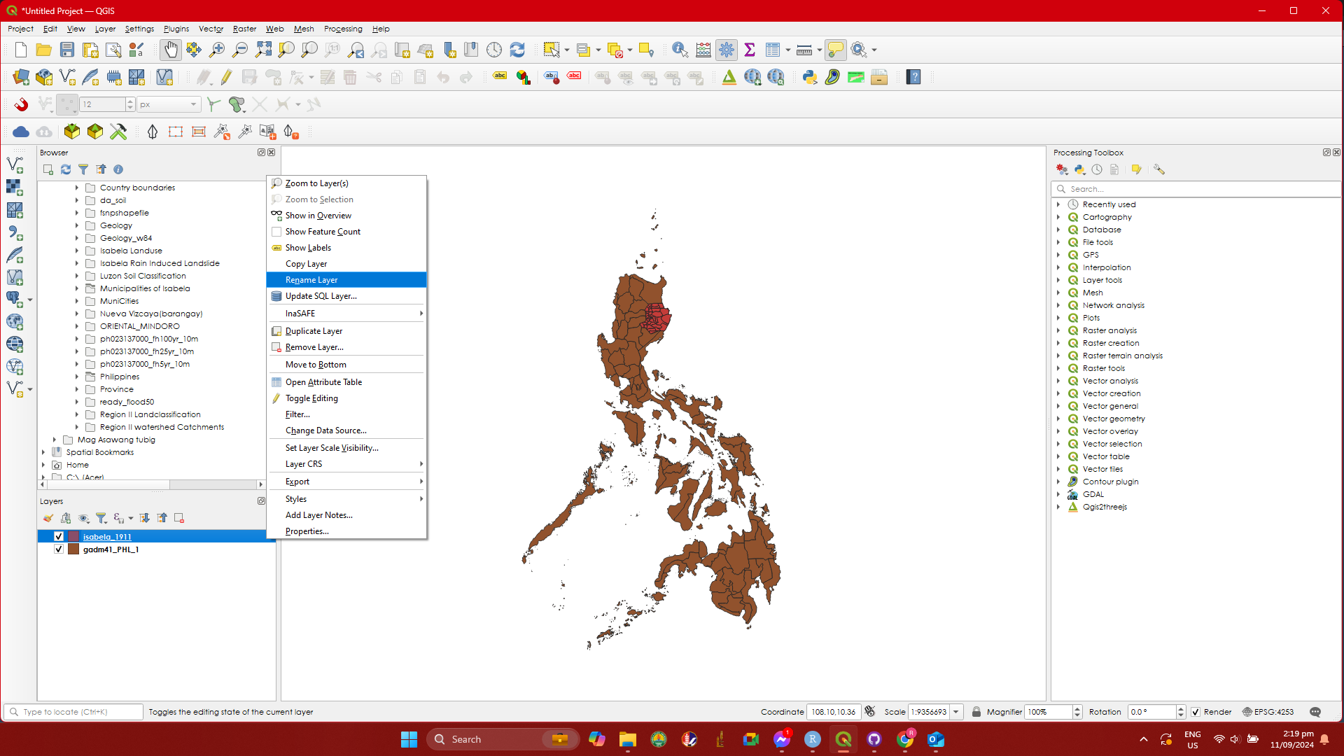
Before opening the Map layout, we should perform some basic styling to our layer. Below some steps on basic styling.
Step 1. First we will do styling on the Isabela_1911 layer. We will change the name of this layer into Municipality of Isabela. To do this, Right click on the Isabela_1911 layer and click Rename Layer then type Municipality of Isabela. Do the same with the gadm41_PHL_1 change it into Regional Boundary.
5 MODULE 5: VECTOR ANALYSIS (Buffer, Clip & Intersection)
5.0.1 Objectives:
This module enables the students to :
Understand vector analysis using the QGIS geoprocessing tools.
Perform Vector analysis using geoprocesing tools.
5.0.2 Outcomes:
After reading and following the steps and procedure in this module, the students should be able to:
Create a buffer zone,
Clip a River lines with Municipal boundary and;
Intersect Raininduce landslide with Municipal boundary.
5.0.3 Buffer
In this exercise, we will learn how to use the buffer tool in QGIS.
When buffering, two areas are created: a buffer zone within a specified distance to selected real-world features and an area beyond it.
A buffer zone is a designated area that exists to maintain distance between different real-world features. These zones can serve a variety of purposes, such as protecting the environment, shielding residential and commercial areas from industrial accidents or natural disasters, or preventing violence. Examples of buffer zones include greenbelts that separate residential and commercial areas, border zones between countries, noise protection zones around airports, and pollution protection zones along rivers.
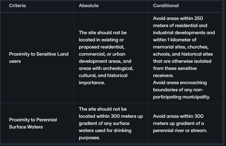
Suppose we are tasked to evaluate an existing sanitary landfill and below is a table showing some of the criteria for evaluation based on DAO 1998-50. We only take two example criteria to show how the buffer tool is used for the evaluation of landfill site identification and screening criteria for municipal solid waste disposal facilities.
Some definition of terms
Absolute criteria - this sets the minimum requirement(s) that a site must meet for it to be considered.
Conditional criteria - this indicates that a certain site has met the absolute Conditions/requirements but is still subject to or dependent upon certain additional conditions that can Enhance the site selection process but are not exclusionary.
As we can see on the first criteria, we need to locate the proposed residential, commercial, or urban development areas, and areas with archeological, cultural, and historical areas. On the second criterion, we need to locate surface waters used for drinking purposes and perennial rivers or streams and of course the location of the existing sanitary landfill. We can obtain these data by digitizing the map.
We will also assume that you have already finished digitizing so that we can now proceed to the validation process using the buffer tool. Download the needed data here.
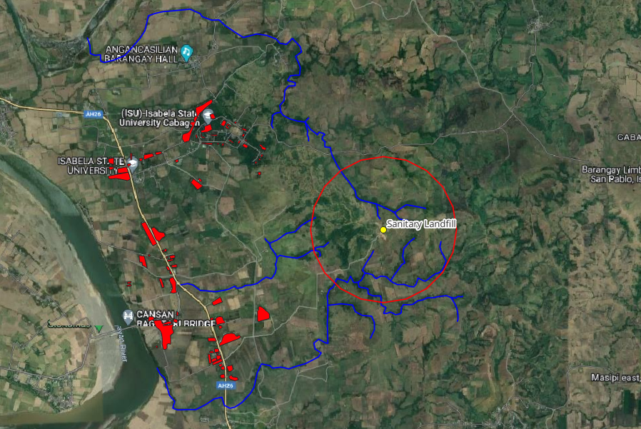
After loading the data within QGIS, we are now ready to evaluate the given criteria. The first criterion says that the landfill should not be located in the proximity of sensitive land users. We can see on the map that the sanitary landfill is situated where there are no built-up areas thus meeting the minimum requirements. However, the conditional states that it should not be within 250 meters of residential and 1 kilometer of memorial sites, churches, schools, and historical sites. To validate this, we will create a 1-kilometer radius buffer zone within the sanitary landfill to see whether there are built-up areas affected.
To create a buffer, follow these steps.
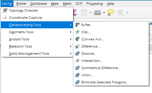
Step 1. In the menu bar, select Vector ---> Geoprocessing tools ---> Buffer.
Step 2. A dialog will appear showing the parameters need to perform the operation.
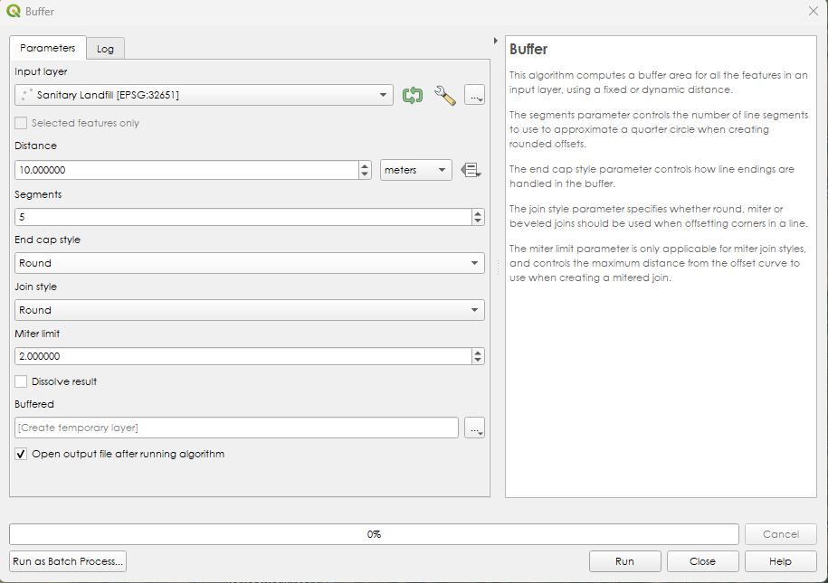
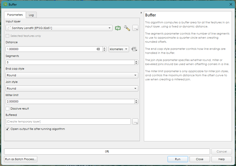
Step 3. On the dialog box, select “Sanitary Landfill” as the Input Layer. On the Distance change the meters into Kilometers and the distance value to 1. Leave other values the same and click Run.
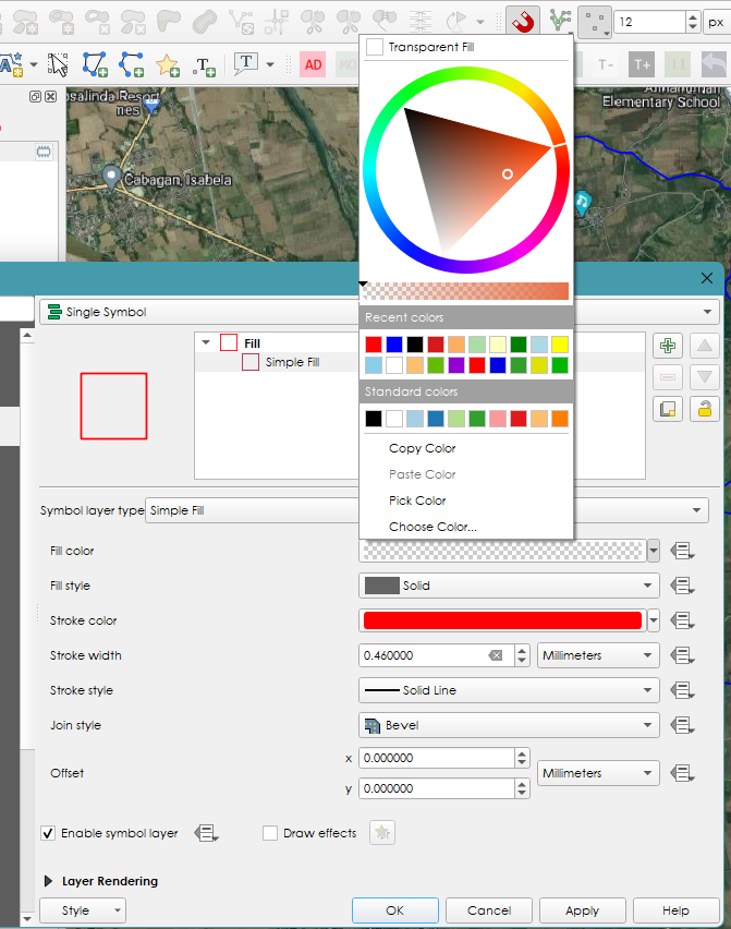
Step 4. A circle will appear around the sanitary landfill. Change the symbology of the buffer zone. Make the fill color to transparent and change the border color into red then increase the stroke width to 0.460000 Click OK.
Step 5. The result shows that there were no built-up areas within the 1-kilometer buffer zone. This means that it passed the first given criteria.
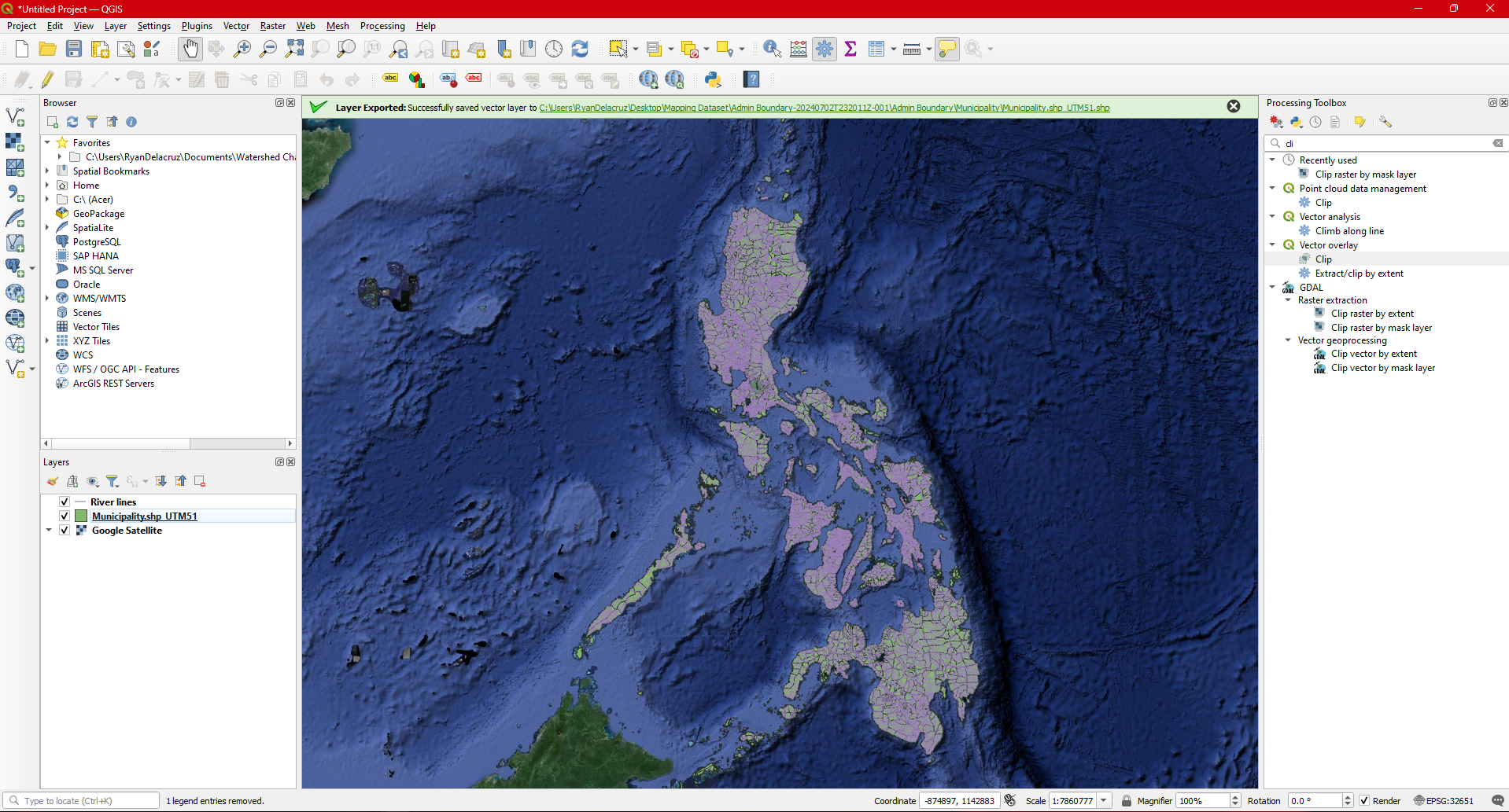
5.0.4 Clip
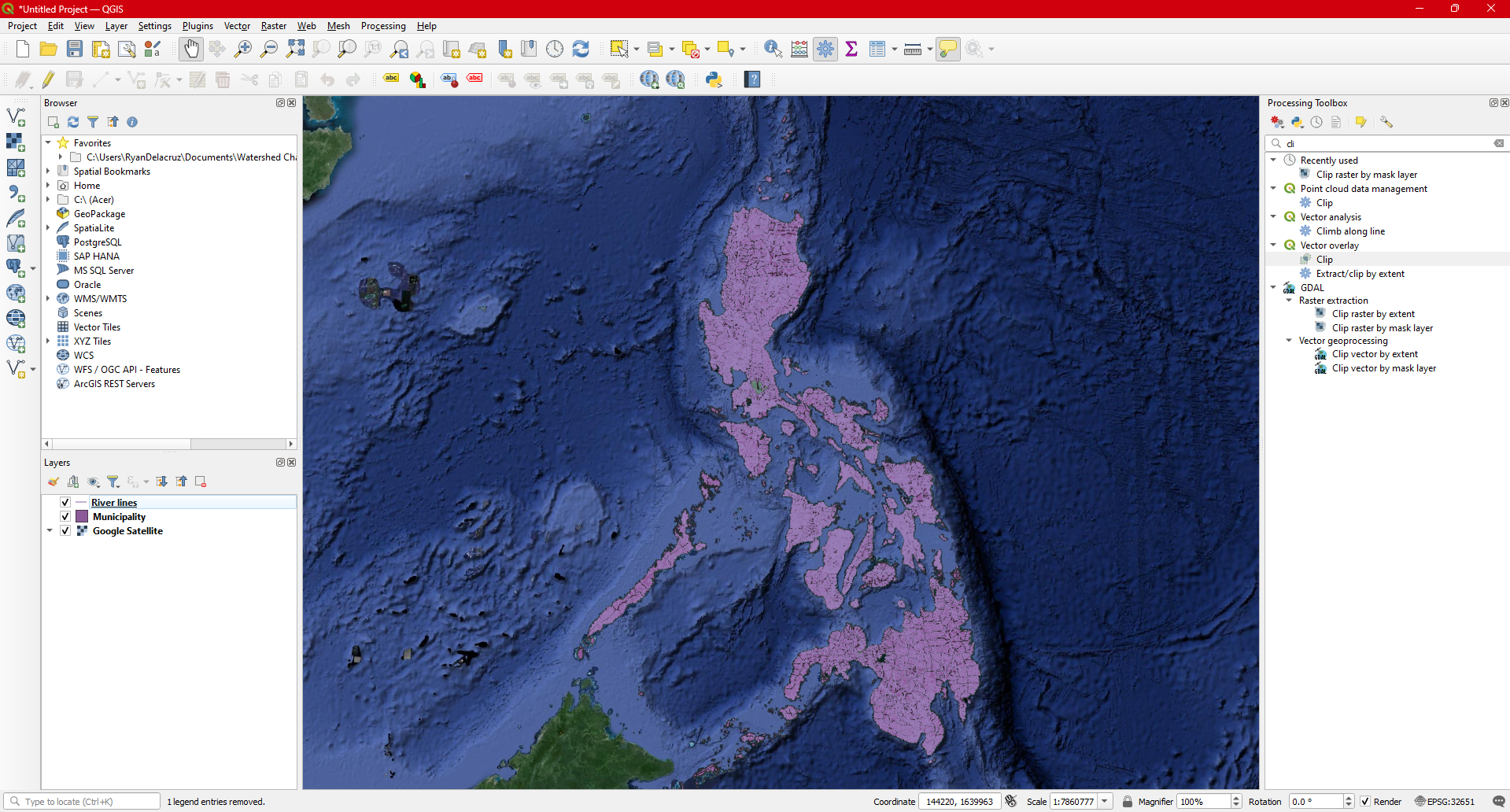
The following steps will guide you on how to perform clipping in QGIS. In this example we will be using the River lines.shp and Municipality.shp
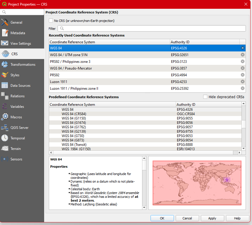
Step 1. Set the project CRS to ESPS:4326-WGS84 . Click  button.
Step 2. Load Municipality.shp using  add vector icon. The same procedure will apply in loading the River lines. shp.
Step 3. Hover your mouse on top each layer to determine their CRS. In our case we can observe that our two layers have different CRS. This is very a important step when you are performing clipping.
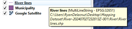
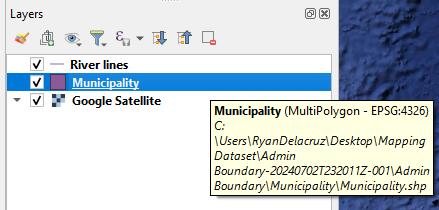
Since the layers have different CRS, you have to export one of the layers to match each others CRS.
If you intended to do an analysis later e.g. Area computation, length etc. it is advisable that you set their CRS to Projected Coordinates. In our case we will set the Municipality.shp to EPSG:32651 since its CRS is Geographic and as we all know its unit is in Degrees.
The following step will guide you on how to do CRS transformation. In some cases these steps may not be necessary specially if your layers have the same CRS. Just proceed to Step 14.
Step 4. Export the Municipality.shp and transform its CRS into EPSG: 32651- UTM51N. To do this Right Click the  in the layers panel and in the menu select
 Export .
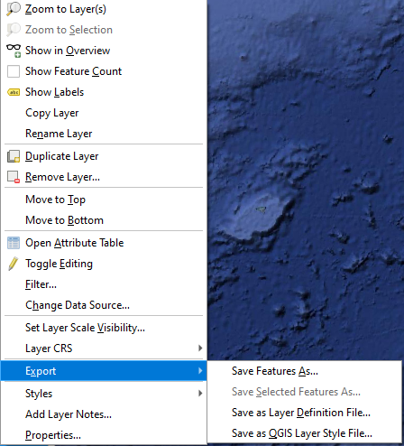
Step 5. Click the  and a dialog box will appear.
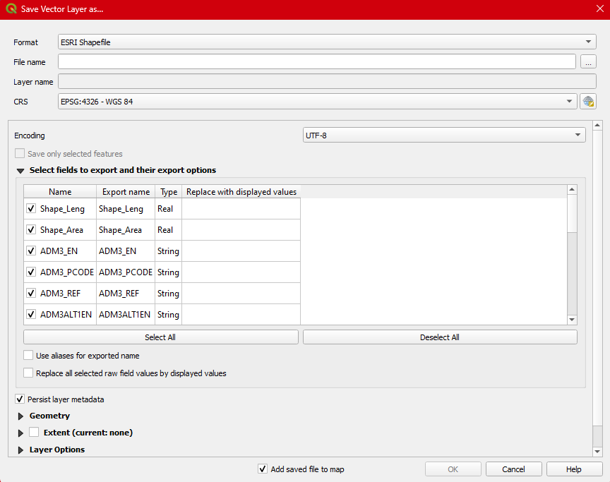
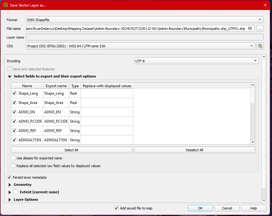
Step 6. Set the Format to ESRI Shapefile . click the  browse button and set the name of the new shapefile to
 Municipality.shp_UTM51. Finally, set the CRS to  . Donforget to Check the
  and hit
 OK .
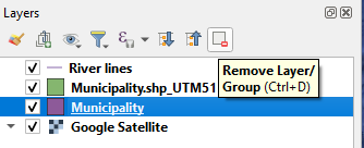
Step 7. Remove the Municipality layer by Clicking it and click  remove layer icon or pressing
 CTRL + D.
Before performing the clipping steps, we will just need to choose a certain municipality and export it. this will help us focus and to make the project clean. So the following steps will show you how to export selected feature from layer.
Step 8. Click the Municipality layer, Right Click to open its 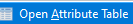 . At the left button part of the dialog box is the
  . Click this button to show some options. Click the
 Field Filter and hit ADM3_EN . This field contains the name of each municipality.
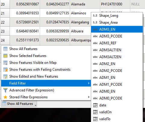
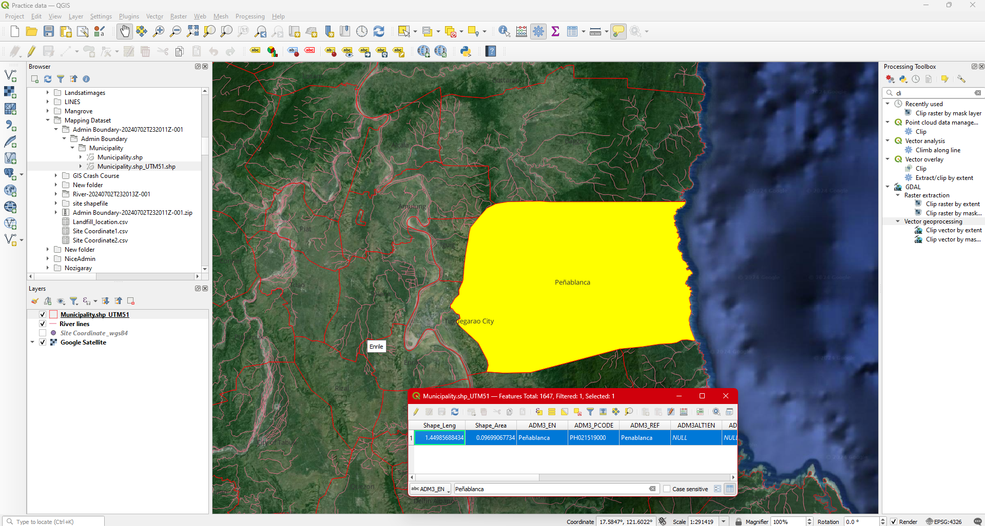
Step 9. In the search bar type the name of the municipality you are interested. In our case, its the municipality of Peñablanca. After typing press Enter on your keyboard,
Step 10. The attribute table will only show the queried name of the municipality. Select the municipality by clicking the id number. You will observed that the selected municipality will be filled with yellow color. This is just an indicator this feature is selected.
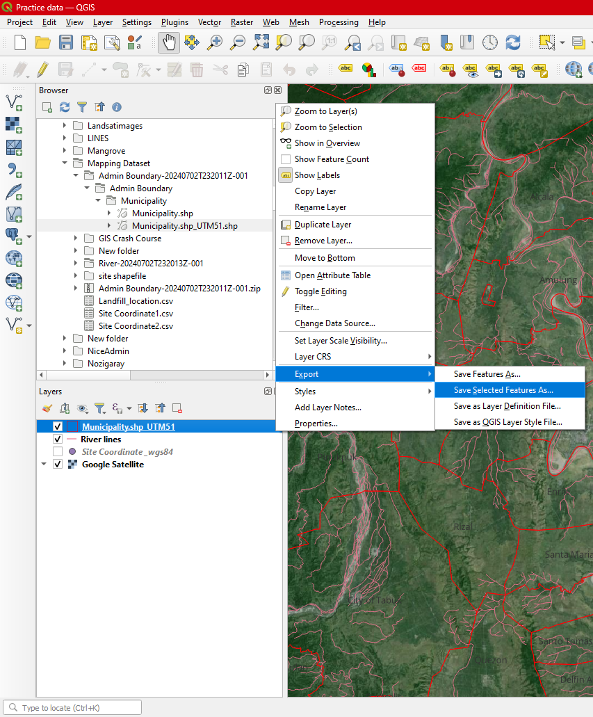
Step 11. Close the attribute table and click the Municipality.shp_UTM51N layer. Right click it then select Export ----> Save Selected feature as .
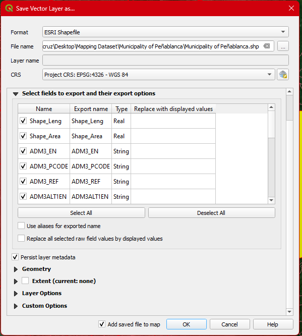
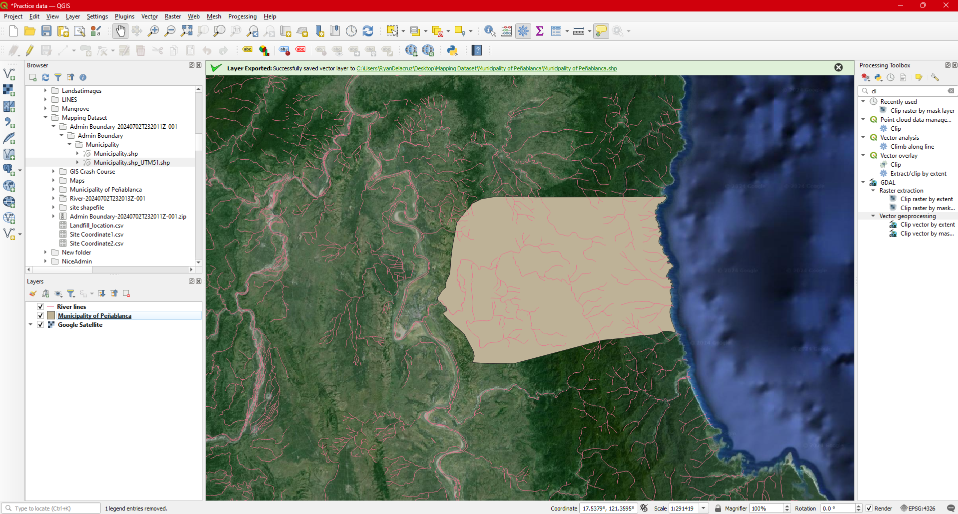
Step 12. In the dialogbox, set Fortmat as ESRI shapefile . Click the browse button and create a folder name Municipality of peñablanca and Save the shapefile as Municipality of Peñablanca.shp. Set the CRS to EPSG: 32651 Don’t forget to check the  to display you output then hit
  .
.
Step 13. Remove the Municipality.shp_UTM51N since we no longer need it for the succeeding steps.
Now we are ready to perform the clipping activity.
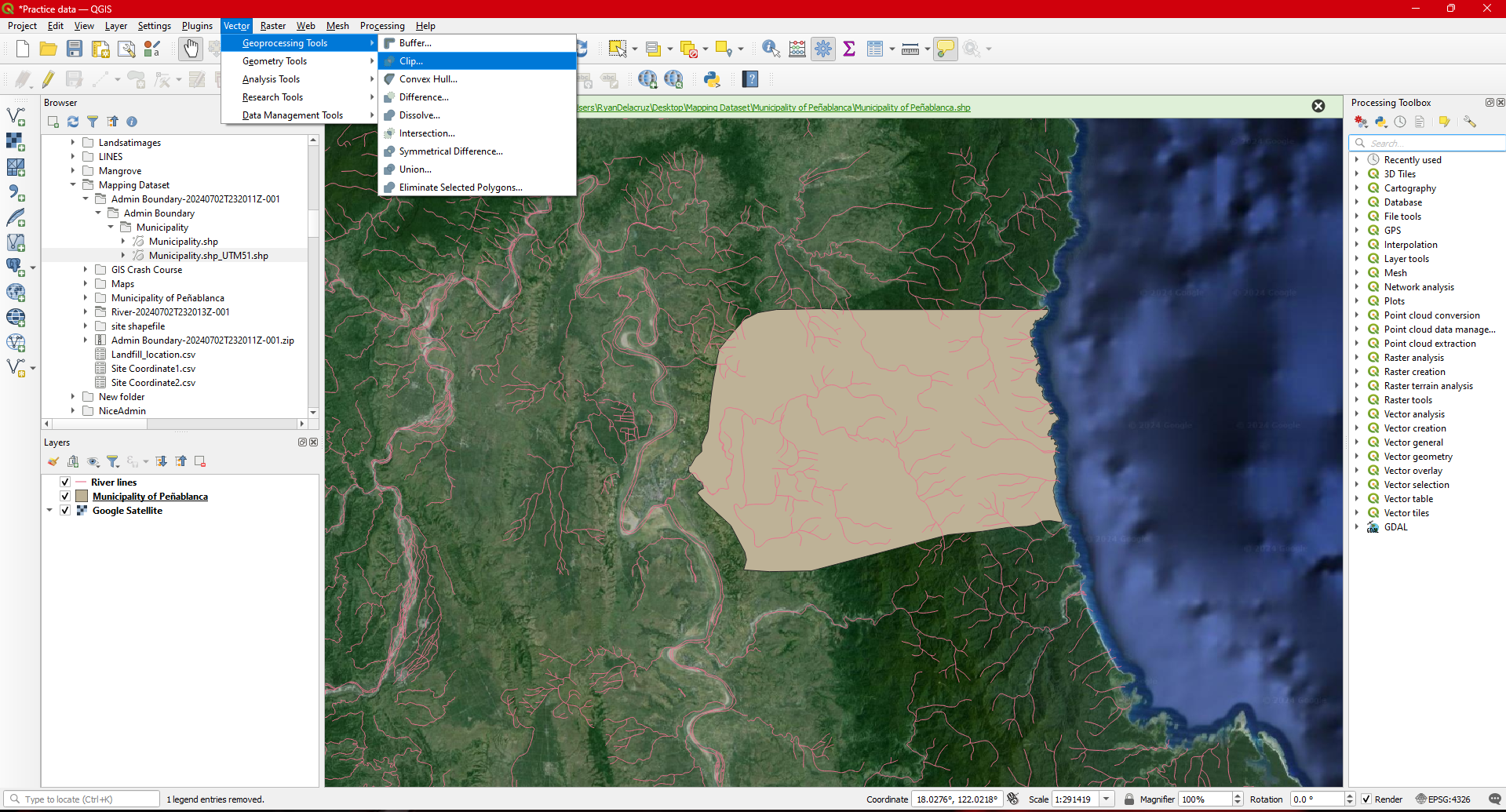
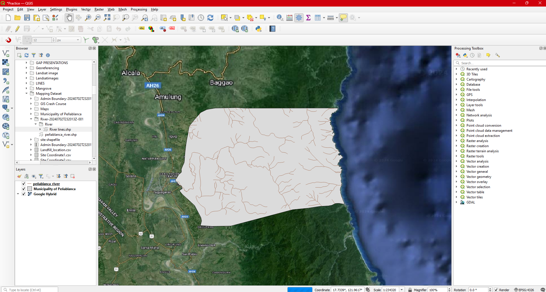
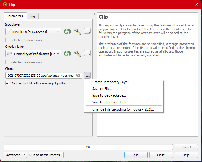
Step 14. Under Vector go to Processing tool the select Clip .
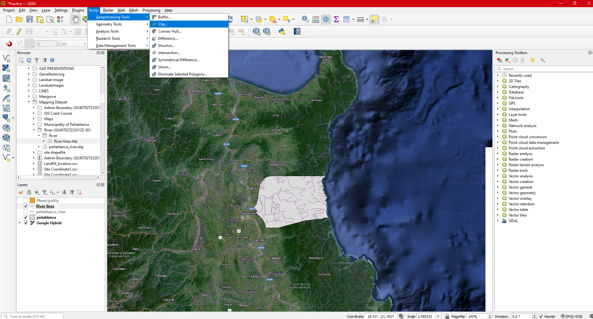
Step 15. In the Input layer select River lines while in the Overly layer select Municipality of Peñblanca. Click the  browse button select
 Save to file and save the shapefile as peñablanca _river. Hit  then
then  .
.
Step 16. Remove River lines from the Layers pannel . You now have the Municipal boundary of Peñablanca and rivers within the municipality.